Creating Decision Trees for Classification Problems - Machine Failure Prediction

General Middleware

March 18, 2023 anbanerj 0 Comment

Creating Decision Trees for Classification Problems – Machine Failure Prediction

Problem Statement

Business Context

System failure is a common issue across the manufacturing industry, where a variety of machines and equipment are used. In most cases, it becomes important to be able to predict machine failures by analyzing system data and taking preventive measures to be able to tackle them. This is known as predictive maintenance and with the rising availability of data and computational resources, the use of such data-driven, proactive maintenance methods has resulted in several benefits like minimized downtime of the equipment, minimized cost associated with spares and supplies, etc.

AutoMobi Engineering Pvt. Ltd is an auto component manufacturing company. The manufacturing facility of AutoMobi consists of numerous products machined on several CNC (Computer Numerical Controlled) machines. In an attempt to transition to a data-driven maintenance process, the company had set up sensors in various locations to collect data regarding the various parameters involved in the manufacturing process. Initially, they want to try it in an injector nozzle manufacturing shop where they are manufacturing fuel injector nozzles for automobile engines using various manufacturing processes (like turning, drilling, etc). The company has been collecting data on an hourly basis from these sensors and aims to build ML-based solutions using the data to optimize cost, improve failure predictability, and minimize the downtime of equipment.

Objective

AutoMobi has recently been encountering a problem with frequent equipment failure in the fuel injector nozzle manufacture unit, leading to disturbance in the manufacturing process. They have reached out to the Data Science team for a solution and shared data for the past three months. As a member of the Data Science team, you are tasked with analyzing the data and developing a Machine Learning model to detect potential machine failures, determine the most influencing factors on machine health, and provide recommendations for cost optimization to the management.

Dataset

Predictive_Maintenance_Case_Study Download

Data Description

The data contains the different attributes of machines and health. The detailed data dictionary is given below.

Data Dictionary

UDI: Unique identifier ranging from 1 to 10000
Type: The type of product consisting of low(60% of all products), medium(30%), and high(10%) quality corresponding to L, M, and H
Air temperature: Ambient temperature (in the machine shop) measured in Kelvin
Process Temperature: Tool tip temperature measured in Kelvin
Rotational Speed: Rotational speed of the machine spindle measured in revolutions per minute (rpm)
Torque: Torque acting on the machine spindle measured in Newton meter (Nm)
Tool wear: Tool wear measured in micrometers (During the manufacturing process, continuous rubbing of the tool on the workpiece leads to the wearing of the tool material. The tool wear is measured as the amount of wear on the cutting face of the tool measured in micrometers)
Failure: 0-No failure, 1-Failure

Importing the necessary libraries

In [ ]:

# this will help in making the Python code more structured automatically (help adhere to good coding practices)
%load_ext nb_black

import warnings
warnings.filterwarnings("ignore")

# Libraries to help with reading and manipulating data
import pandas as pd
import numpy as np

# libaries to help with data visualization
import matplotlib.pyplot as plt
import seaborn as sns

# Removes the limit for the number of displayed columns
pd.set_option("display.max_columns", None)
# Sets the limit for the number of displayed rows
pd.set_option("display.max_rows", 200)
# setting the precision of floating numbers to 5 decimal points
pd.set_option("display.float_format", lambda x: "%.5f" % x)

# Library to split data
from sklearn.model_selection import train_test_split

# To build model for prediction
from sklearn.tree import DecisionTreeClassifier
from sklearn import tree

# To tune different models
from sklearn.model_selection import GridSearchCV

# To get diferent metric scores
from sklearn.metrics import (
    f1_score,
    accuracy_score,
    recall_score,
    precision_score,
    confusion_matrix,
    make_scorer,
)

Loading the dataset

In [ ]:

df_main = pd.read_csv("Predictive_Maintenance_Case_Study.csv")

In [ ]:

# copying data to another variable to avoid any changes to original data
data = df_main.copy()

Overview of the dataset

View the first and last 5 rows of the dataset.

In [ ]:

data.head()

Out[ ]:

	UDI	Type	Air temperature	Process temperature	Rotational speed	Torque	Tool wear
0	1	M	298.10000	323.74074	1551	42.80000	0
1	2	L	298.20000	324.11111	1408	46.30000	3
2	3	L	298.10000	323.37037	1498	49.40000	5
3	4	L	298.20000	323.74074	1433	39.50000	7
4	5	L	298.20000	324.11111	1408	40.00000	9

In [ ]:

data.tail()

Out[ ]:

	UDI	Type	Air temperature	Process temperature	Rotational speed	Torque	Tool wear
9995	9996	M	298.80000	323.00000	1604	29.50000	14
9996	9997	H	298.90000	323.00000	1632	31.80000	17
9997	9998	M	299.00000	323.74074	1645	33.40000	22
9998	9999	H	299.00000	324.11111	1408	48.50000	25
9999	10000	M	299.00000	324.11111	1500	40.20000	30

There are three types of products those are L, M, and H (Low, Medium, and High quality).
The UDI column is containing unique values.

Understand the shape of the dataset.

In [ ]:

data.shape

Out[ ]:

(10000, 8)

The dataset has 10000 rows and 8 columns.

Check the data types of the columns for the dataset.

In [ ]:

data.info()

<class 'pandas.core.frame.DataFrame'>
RangeIndex: 10000 entries, 0 to 9999
Data columns (total 8 columns):
 #   Column               Non-Null Count  Dtype  
---  ------               --------------  -----  
 0   UDI                  10000 non-null  int64  
 1   Type                 10000 non-null  object 
 2   Air temperature      10000 non-null  float64
 3   Process temperature  10000 non-null  float64
 4   Rotational speed     10000 non-null  int64  
 5   Torque               10000 non-null  float64
 6   Tool wear            10000 non-null  int64  
 7   Failure              10000 non-null  int64  
dtypes: float64(3), int64(4), object(1)
memory usage: 625.1+ KB

The Type column is of object type while the rest columns are numeric in nature

Checking for missing values

In [ ]:

# checking for null values
data.isnull().sum()

Out[ ]:

UDI                    0
Type                   0
Air temperature        0
Process temperature    0
Rotational speed       0
Torque                 0
Tool wear              0
Failure                0
dtype: int64

There are no null values in the dataset

Dropping the duplicate values

In [ ]:

# checking for duplicate values
data.duplicated().sum()

Out[ ]:

There are no duplicate values in the data.

Dropping the columns with all unique values

In [ ]:

data.UDI.nunique()

Out[ ]:

The UDI column contains only unique values, so we can drop it

In [ ]:

data = data.drop(["UDI"], axis=1)

Statistical summary of the data

Let’s check the statistical summary of the data.

In [ ]:

data.describe().T

Out[ ]:

	count	mean	std	min	25%	50%	75%	max
Air temperature	10000.00000	300.00493	2.00026	295.30000	298.30000	300.10000	301.50000	304.50000
Process temperature	10000.00000	328.94652	5.49531	313.00000	324.48148	329.29630	333.00000	343.00000
Rotational speed	10000.00000	1538.77610	179.28410	1168.00000	1423.00000	1503.00000	1612.00000	2886.00000
Torque	10000.00000	39.98691	9.96893	3.80000	33.20000	40.10000	46.80000	76.60000
Tool wear	10000.00000	107.95100	63.65415	0.00000	53.00000	108.00000	162.00000	253.00000
Failure	10000.00000	0.03390	0.18098	0.00000	0.00000	0.00000	0.00000	1.00000

The air temperature ranges from 300K to 304.5K. Usually, machine shops are maintained in control environment so the temperature range looks usual.
The process temperature is a bit higher than the air temperature and that’s quite usual because heat is continuously generated during the machining process.
The rotational speed has a max value of 2886rpm while 1612rpm at the 75th percentile. Some of the processes are performed at a higher speed than usual.

Exploratory Data Analysis (EDA) Summary

Note: The EDA section has been covered multiple times in the previous case studies. In this case study, we will mainly focus on the model building aspects. We will only be looking at the key observations from EDA. The detailed EDA can be found in the appendix section.

The below functions need to be defined to carry out the EDA.

In [ ]:

def histogram_boxplot(data, feature, figsize=(15, 10), kde=False, bins=None):
    """
    Boxplot and histogram combined

    data: dataframe
    feature: dataframe column
    figsize: size of figure (default (15,10))
    kde: whether to show the density curve (default False)
    bins: number of bins for histogram (default None)
    """
    f2, (ax_box2, ax_hist2) = plt.subplots(
        nrows=2,  # Number of rows of the subplot grid= 2
        sharex=True,  # x-axis will be shared among all subplots
        gridspec_kw={"height_ratios": (0.25, 0.75)},
        figsize=figsize,
    )  # creating the 2 subplots
    sns.boxplot(
        data=data, x=feature, ax=ax_box2, showmeans=True, color="violet"
    )  # boxplot will be created and a triangle will indicate the mean value of the column
    sns.histplot(
        data=data, x=feature, kde=kde, ax=ax_hist2, bins=bins
    ) if bins else sns.histplot(
        data=data, x=feature, kde=kde, ax=ax_hist2
    )  # For histogram
    ax_hist2.axvline(
        data[feature].mean(), color="green", linestyle="--"
    )  # Add mean to the histogram
    ax_hist2.axvline(
        data[feature].median(), color="black", linestyle="-"
    )  # Add median to the histogram

In [ ]:

# function to create labeled barplots


def labeled_barplot(data, feature, perc=False, n=None):
    """
    Barplot with percentage at the top

    data: dataframe
    feature: dataframe column
    perc: whether to display percentages instead of count (default is False)
    n: displays the top n category levels (default is None, i.e., display all levels)
    """

    total = len(data[feature])  # length of the column
    count = data[feature].nunique()
    if n is None:
        plt.figure(figsize=(count + 2, 6))
    else:
        plt.figure(figsize=(n + 2, 6))

    plt.xticks(rotation=90, fontsize=15)
    ax = sns.countplot(
        data=data,
        x=feature,
        palette="Paired",
        order=data[feature].value_counts().index[:n],
    )

    for p in ax.patches:
        if perc == True:
            label = "{:.1f}%".format(
                100 * p.get_height() / total
            )  # percentage of each class of the category
        else:
            label = p.get_height()  # count of each level of the category

        x = p.get_x() + p.get_width() / 2  # width of the plot
        y = p.get_height()  # height of the plot

        ax.annotate(
            label,
            (x, y),
            ha="center",
            va="center",
            size=12,
            xytext=(0, 5),
            textcoords="offset points",
        )  # annotate the percentage

    plt.show()  # show the plot

In [ ]:

def stacked_barplot(data, predictor, target):
    """
    Print the category counts and plot a stacked bar chart

    data: dataframe
    predictor: independent variable
    target: target variable
    """
    count = data[predictor].nunique()
    sorter = data[target].value_counts().index[-1]
    tab1 = pd.crosstab(data[predictor], data[target], margins=True).sort_values(
        by=sorter, ascending=False
    )
    print(tab1)
    print("-" * 120)
    tab = pd.crosstab(data[predictor], data[target], normalize="index").sort_values(
        by=sorter, ascending=False
    )
    tab.plot(kind="bar", stacked=True, figsize=(count + 5, 5))
    plt.legend(
        loc="lower left", frameon=False,
    )
    plt.legend(loc="upper left", bbox_to_anchor=(1, 1))
    plt.show()

In [ ]:

### function to plot distributions wrt target


def distribution_plot_wrt_target(data, predictor, target):

    fig, axs = plt.subplots(2, 2, figsize=(12, 10))

    target_uniq = data[target].unique()

    axs[0, 0].set_title("Distribution of target for target=" + str(target_uniq[0]))
    sns.histplot(
        data=data[data[target] == target_uniq[0]],
        x=predictor,
        kde=True,
        ax=axs[0, 0],
        color="teal",
        stat="density",
    )

    axs[0, 1].set_title("Distribution of target for target=" + str(target_uniq[1]))
    sns.histplot(
        data=data[data[target] == target_uniq[1]],
        x=predictor,
        kde=True,
        ax=axs[0, 1],
        color="orange",
        stat="density",
    )

    axs[1, 0].set_title("Boxplot w.r.t target")
    sns.boxplot(data=data, x=target, y=predictor, ax=axs[1, 0], palette="gist_rainbow")

    axs[1, 1].set_title("Boxplot (without outliers) w.r.t target")
    sns.boxplot(
        data=data,
        x=target,
        y=predictor,
        ax=axs[1, 1],
        showfliers=False,
        palette="gist_rainbow",
    )

    plt.tight_layout()
    plt.show()

Univariate Analysis

In [ ]:

histogram_boxplot(data, "Air temperature")

The air temperature distribution looks slightly left skewed with a mean temperature around 300K.
There is no outlier present.

In [ ]:

histogram_boxplot(data, "Process temperature")

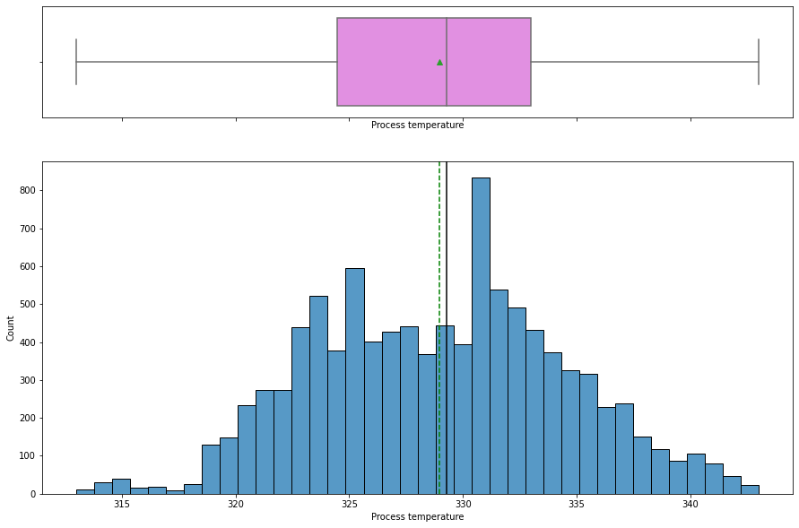
The process temperature distribution looks slightly left skewed with a mean temperature around 329K.
There is no outlier present.

In [ ]:

histogram_boxplot(data, "Rotational speed")

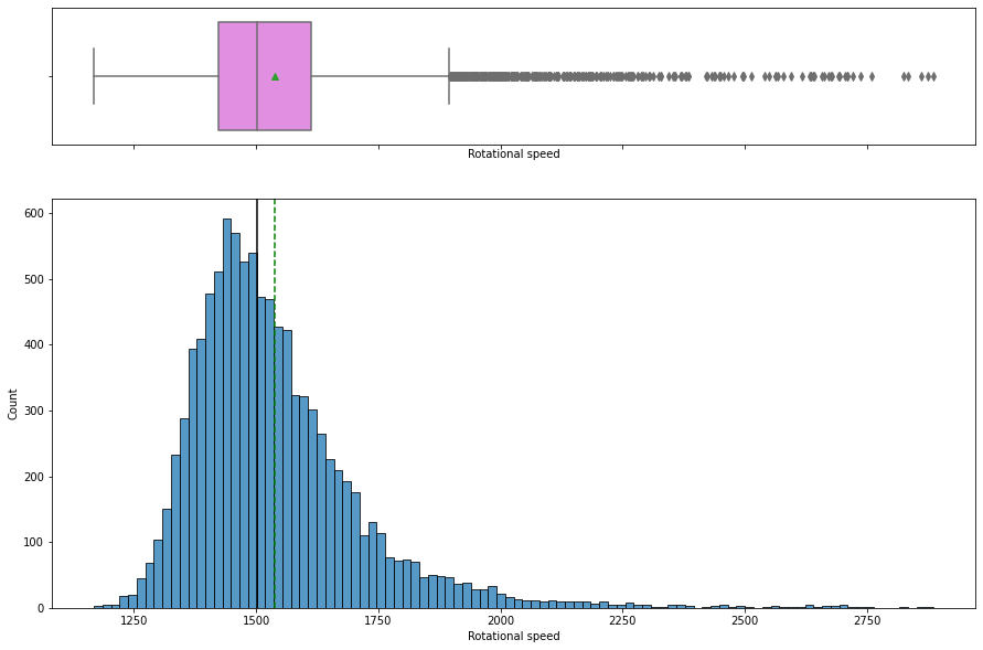
The rotational speed is right skewed with many outliers on the upper quartile.
Some of the manufacturing operations are performed at a higher speed.

In [ ]:

histogram_boxplot(data, "Torque")

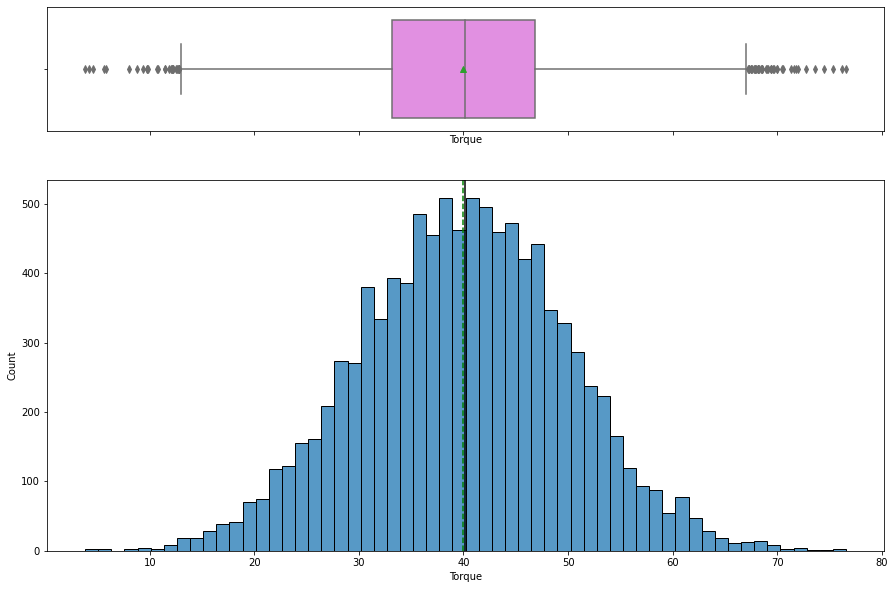
The distribution of torque is normal with mean torque around 40 Nm.
Outliers are present on both sides.

In [ ]:

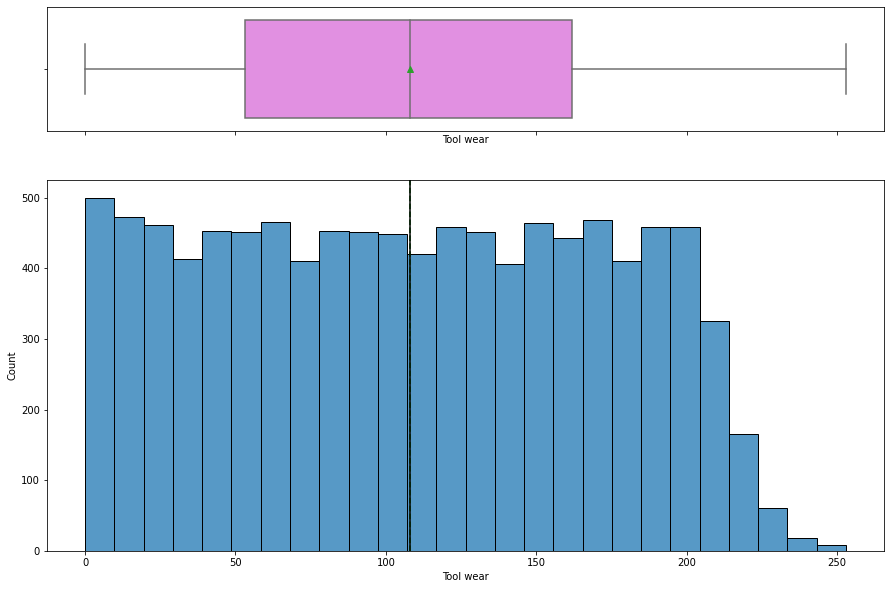
histogram_boxplot(data, "Tool wear")

Tool wear is uniformly distributed with some of the higher values being less frequent.

In [ ]:

labeled_barplot(data, "Type", perc=True)

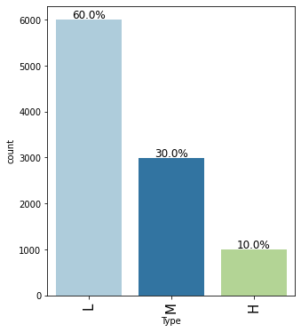
Around 60% of products are of low quality, 30% are of medium quality whereas 10% are of high quality

In [ ]:

labeled_barplot(data, "Failure", perc=True)

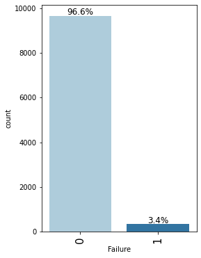
In 96.6% of observations the machine does not fail while in 3.4% of observations it fails.

Bivariate Analysis

In [ ]:

cols_list = data.select_dtypes(include=np.number).columns.tolist()
cols_list.remove('Failure')

plt.figure(figsize=(12, 7))
sns.heatmap(
    data[cols_list].corr(), annot=True, vmin=-1, vmax=1, fmt=".2f", cmap="Spectral"
)
plt.show()

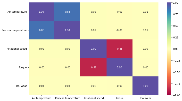
There’s a positive correlation between the air temperature and process temperature.
There’s a negative correlation between the rotational speed and torque.
No other variables are correlated. We will analyze it further.

Let’s see how the target variable varies across the type of the product

In [ ]:

stacked_barplot(data, "Type", "Failure")

Failure     0    1    All
Type                     
All      9661  339  10000
L        5765  235   6000
M        2914   83   2997
H         982   21   1003
------------------------------------------------------------------------------------------------------------------------

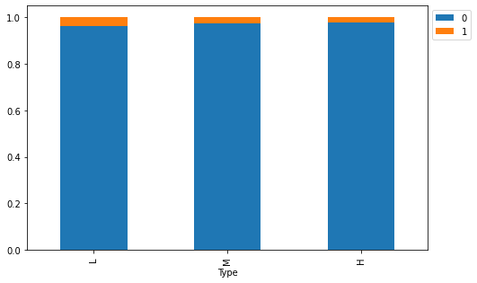
Around 70 % of the failure occurred during machining of L type i.e., low-quality products.
Machining of high-quality products is less prone to failure.

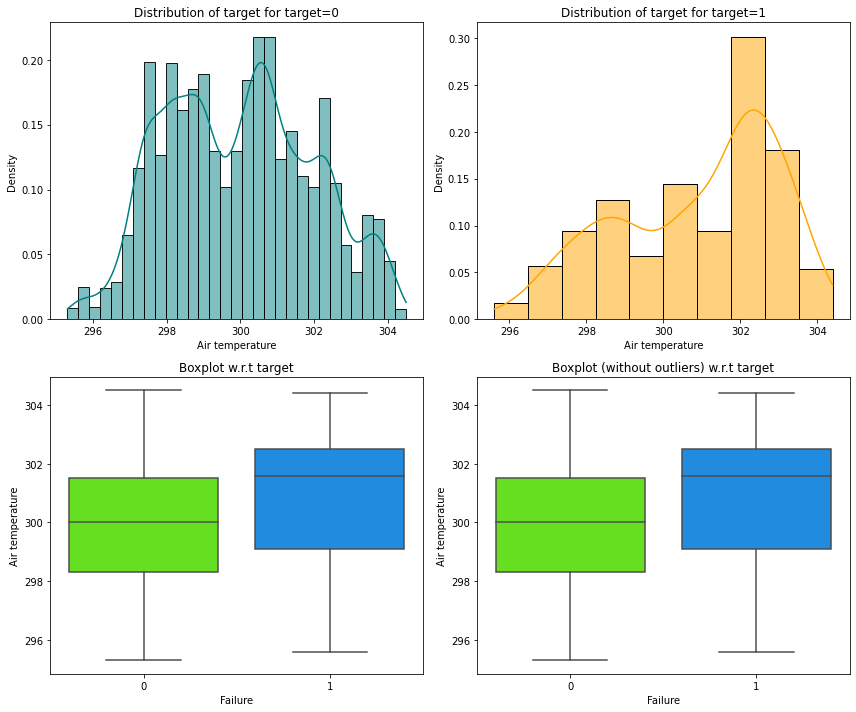
Let’s analyze the relation between Process temperature and Failure.

In [ ]:

distribution_plot_wrt_target(data, "Process temperature", "Failure")

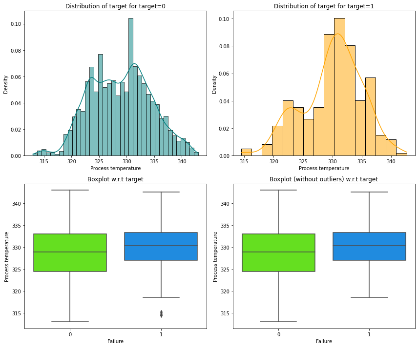
Most of the failures of the manufacturing system occur at higher Process temperature.

Let’s analyze the relation between Rotational speed and Failure.

In [ ]:

distribution_plot_wrt_target(data, "Rotational speed", "Failure")

There is a clear boundary showing separation of failure status based of the values of Rotational speed.
Manufacturing system is more prone to failure at lower Rotational speed than at higher rotational speed.

Data Preprocessing

Outlier Detection

Let’s check for outliers in the data.

In [ ]:

# outlier detection using boxplot
numeric_columns = data.select_dtypes(include=np.number).columns.tolist()

plt.figure(figsize=(15, 12))

for i, variable in enumerate(numeric_columns):
    plt.subplot(4, 4, i + 1)
    plt.boxplot(data[variable], whis=1.5)
    plt.tight_layout()
    plt.title(variable)

plt.show()

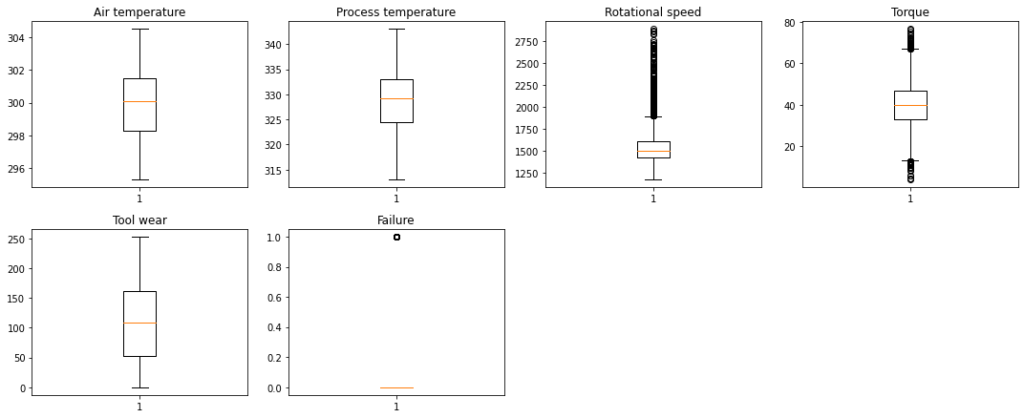
Observations

There are quite a few outliers in the data.
However, we will not treat them as they are proper values

Data Preparation for Modeling

In [ ]:

X = data.drop(["Failure"], axis=1)
Y = data["Failure"]

X = pd.get_dummies(X, drop_first=True)

# Splitting data in train and test sets
X_train, X_test, y_train, y_test = train_test_split(
    X, Y, test_size=0.30, random_state=1
)

In [ ]:

print("Shape of Training set : ", X_train.shape)
print("Shape of test set : ", X_test.shape)
print("Percentage of classes in training set:")
print(y_train.value_counts(normalize=True))
print("Percentage of classes in test set:")
print(y_test.value_counts(normalize=True))

Shape of Training set :  (7000, 7)
Shape of test set :  (3000, 7)
Percentage of classes in training set:
0   0.96629
1   0.03371
Name: Failure, dtype: float64
Percentage of classes in test set:
0   0.96567
1   0.03433
Name: Failure, dtype: float64

We had seen that around 96.6% of observations belongs to class 0 (Not Failed) and 3.37% observations belongs to class 1 (Failed), and this is preserved in the train and test sets

Model Building

Decision Tree (default)

In [ ]:

model0 = DecisionTreeClassifier(random_state=1)
model0.fit(X_train, y_train)

Out[ ]:

DecisionTreeClassifier(random_state=1)

Model Evaluation

Model evaluation criterion

Model can make wrong predictions as:

Predicting a machine will not fail but in reality, the machine will fail (FN)
Predicting a machine will fail but in reality, the machine will not fail (FP)

Which case is more important?

If we predict that a machine will not fail but in reality, the machine fails, then the company will have to bear the cost of repair/replacement and also face equipment downtime losses
If we predict that a machine will fail but in reality, the machine does not fail, then the company will have to bear the cost of inspection
The inspection cost is generally less compared to the repair/replacement cost

How to reduce the losses?

The company would want the recall to be maximized, greater the recall score higher are the chances of minimizing the False Negatives.

In [ ]:

# defining a function to compute different metrics to check performance of a classification model built using sklearn
def model_performance_classification_sklearn(model, predictors, target):
    """
    Function to compute different metrics to check classification model performance

    model: classifier
    predictors: independent variables
    target: dependent variable
    """

    # predicting using the independent variables
    pred = model.predict(predictors)

    acc = accuracy_score(target, pred)  # to compute Accuracy
    recall = recall_score(target, pred)  # to compute Recall
    precision = precision_score(target, pred)  # to compute Precision
    f1 = f1_score(target, pred)  # to compute F1-score

    # creating a dataframe of metrics
    df_perf = pd.DataFrame(
        {"Accuracy": acc, "Recall": recall, "Precision": precision, "F1": f1,},
        index=[0],
    )

    return df_perf

In [ ]:

def confusion_matrix_sklearn(model, predictors, target):
    """
    To plot the confusion_matrix with percentages

    model: classifier
    predictors: independent variables
    target: dependent variable
    """
    y_pred = model.predict(predictors)
    cm = confusion_matrix(target, y_pred)
    labels = np.asarray(
        [
            ["{0:0.0f}".format(item) + "\n{0:.2%}".format(item / cm.flatten().sum())]
            for item in cm.flatten()
        ]
    ).reshape(2, 2)

    plt.figure(figsize=(6, 4))
    sns.heatmap(cm, annot=labels, fmt="")
    plt.ylabel("True label")
    plt.xlabel("Predicted label")

In [ ]:

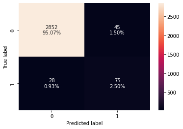
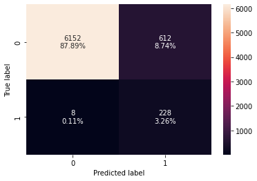
confusion_matrix_sklearn(model0, X_train, y_train)

In [ ]:

decision_tree_perf_train_without = model_performance_classification_sklearn(
    model0, X_train, y_train
)
decision_tree_perf_train_without

Out[ ]:

	Accuracy	Recall	Precision	F1
0	1.00000	1.00000	1.00000	1.00000

In [ ]:

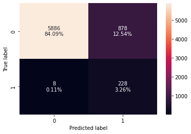
confusion_matrix_sklearn(model0, X_test, y_test)

In [ ]:

decision_tree_perf_test_without = model_performance_classification_sklearn(
    model0, X_test, y_test
)
decision_tree_perf_test_without

Out[ ]:

	Accuracy	Recall	Precision	F1
0	0.97567	0.72816	0.62500	0.67265

Decision Tree (with class_weights)

If the frequency of class A is 10% and the frequency of class B is 90%, then class B will become the dominant class and the decision tree will become biased toward the dominant classes
In this case, we will set class_weight = “balanced”, which will automatically adjust the weights to be inversely proportional to the class frequencies in the input data
class_weight is a hyperparameter for the decision tree classifier

In [ ]:

model = DecisionTreeClassifier(random_state=1, class_weight="balanced")
model.fit(X_train, y_train)

Out[ ]:

DecisionTreeClassifier(class_weight='balanced', random_state=1)

In [ ]:

confusion_matrix_sklearn(model, X_train, y_train)

In [ ]:

decision_tree_perf_train = model_performance_classification_sklearn(
    model, X_train, y_train
)
decision_tree_perf_train

Out[ ]:

	Accuracy	Recall	Precision	F1
0	1.00000	1.00000	1.00000	1.00000

Model is able to perfectly classify all the data points on the training set.
0 errors on the training set, each sample has been classified correctly.
As we know a decision tree will continue to grow and classify each data point correctly if no restrictions are applied as the trees will learn all the patterns in the training set.
This generally leads to overfitting of the model as Decision Tree will perform well on the training set but will fail to replicate the performance on the test set.

In [ ]:

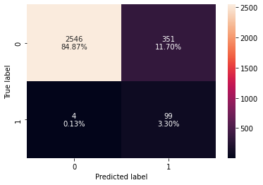
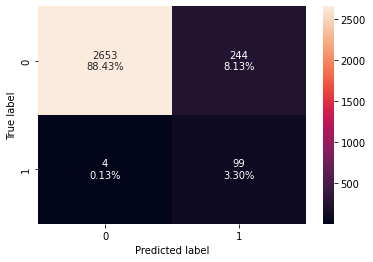
confusion_matrix_sklearn(model, X_test, y_test)

In [ ]:

decision_tree_perf_test = model_performance_classification_sklearn(
    model, X_test, y_test
)
decision_tree_perf_test

Out[ ]:

	Accuracy	Recall	Precision	F1
0	0.97700	0.61165	0.68478	0.64615

There is a huge disparity in performance of model on training set and test set, which suggests that the model is overfiiting.

Let’s use pruning techniques to try and reduce overfitting.

Decision Tree (Pre-pruning)

Using GridSearch for Hyperparameter tuning of our tree model

Hyperparameter tuning is also tricky in the sense that there is no direct way to calculate how a change in the hyperparameter value will reduce the loss of your model, so we usually resort to experimentation. i.e we’ll use Grid search
Grid search is a tuning technique that attempts to compute the optimum values of hyperparameters.
It is an exhaustive search that is performed on a the specific parameter values of a model.
The parameters of the estimator/model used to apply these methods are optimized by cross-validated grid-search over a parameter grid.

In [ ]:

# Choose the type of classifier.
estimator = DecisionTreeClassifier(random_state=1)

# Grid of parameters to choose from
parameters = {
    "class_weight": [None, "balanced"],
    "max_depth": np.arange(2, 7, 2),
    "max_leaf_nodes": [50, 75, 150, 250],
    "min_samples_split": [10, 30, 50, 70],
}

# Type of scoring used to compare parameter combinations
acc_scorer = make_scorer(recall_score)

# Run the grid search
grid_obj = GridSearchCV(estimator, parameters, scoring=acc_scorer, cv=5)
grid_obj = grid_obj.fit(X_train, y_train)

# Set the clf to the best combination of parameters
estimator = grid_obj.best_estimator_

# Fit the best algorithm to the data.
estimator.fit(X_train, y_train)

Out[ ]:

DecisionTreeClassifier(class_weight='balanced', max_depth=4, max_leaf_nodes=50,
                       min_samples_split=70, random_state=1)

In [ ]:

confusion_matrix_sklearn(estimator, X_train, y_train)

In [ ]:

decision_tree_tune_perf_train = model_performance_classification_sklearn(
    estimator, X_train, y_train
)
decision_tree_tune_perf_train

Out[ ]:

	Accuracy	Recall	Precision	F1
0	0.87343	0.96610	0.20615	0.33979

In [ ]:

confusion_matrix_sklearn(estimator, X_test, y_test)

In [ ]:

decision_tree_tune_perf_test = model_performance_classification_sklearn(
    estimator, X_test, y_test
)
decision_tree_tune_perf_test

Out[ ]:

	Accuracy	Recall	Precision	F1
0	0.88167	0.96117	0.22000	0.35805

The model is giving a generalized result now since the recall scores on both the train and test data are coming to be around 0.96 which shows that the model is able to generalize well on unseen data.

In [ ]:

feature_names = list(X_train.columns)
importances = estimator.feature_importances_
indices = np.argsort(importances)

In [ ]:

plt.figure(figsize=(20, 10))
out = tree.plot_tree(
    estimator,
    feature_names=feature_names,
    filled=True,
    fontsize=9,
    node_ids=False,
    class_names=None,
)
# below code will add arrows to the decision tree split if they are missing
for o in out:
    arrow = o.arrow_patch
    if arrow is not None:
        arrow.set_edgecolor("black")
        arrow.set_linewidth(1)
plt.show()

In [ ]:

# Text report showing the rules of a decision tree -
print(tree.export_text(estimator, feature_names=feature_names, show_weights=True))

|--- Rotational speed <= 1379.50
|   |--- Air temperature <= 301.55
|   |   |--- Torque <= 52.85
|   |   |   |--- Tool wear <= 206.50
|   |   |   |   |--- weights: [176.97, 0.00] class: 0
|   |   |   |--- Tool wear >  206.50
|   |   |   |   |--- weights: [10.35, 59.32] class: 1
|   |   |--- Torque >  52.85
|   |   |   |--- Tool wear <= 185.50
|   |   |   |   |--- weights: [151.61, 341.10] class: 1
|   |   |   |--- Tool wear >  185.50
|   |   |   |   |--- weights: [9.31, 474.58] class: 1
|   |--- Air temperature >  301.55
|   |   |--- Process temperature <= 336.89
|   |   |   |--- Process temperature <= 330.96
|   |   |   |   |--- weights: [1.03, 504.24] class: 1
|   |   |   |--- Process temperature >  330.96
|   |   |   |   |--- weights: [42.95, 845.34] class: 1
|   |   |--- Process temperature >  336.89
|   |   |   |--- weights: [32.08, 59.32] class: 1
|--- Rotational speed >  1379.50
|   |--- Tool wear <= 202.50
|   |   |--- Torque <= 15.45
|   |   |   |--- weights: [11.90, 281.78] class: 1
|   |   |--- Torque >  15.45
|   |   |   |--- Torque <= 58.40
|   |   |   |   |--- weights: [2865.61, 118.64] class: 0
|   |   |   |--- Torque >  58.40
|   |   |   |   |--- weights: [5.69, 177.97] class: 1
|   |--- Tool wear >  202.50
|   |   |--- Tool wear <= 219.50
|   |   |   |--- Torque <= 51.85
|   |   |   |   |--- weights: [154.72, 311.44] class: 1
|   |   |   |--- Torque >  51.85
|   |   |   |   |--- weights: [2.59, 59.32] class: 1
|   |   |--- Tool wear >  219.50
|   |   |   |--- Air temperature <= 297.20
|   |   |   |   |--- weights: [3.10, 0.00] class: 0
|   |   |   |--- Air temperature >  297.20
|   |   |   |   |--- weights: [32.08, 266.95] class: 1

Observations from the pre-pruned tree:

Using the above extracted decision rules we can make interpretations from the decision tree model like:

If the rotational speed is less than or equal to 1379.50, the air temperature is less than or equal to 301.55, the torque is less than or equal to 52.85 and the tool wear is greater than 206.50, then the machine is most likey to fail

Interpretations from other decision rules can be made similarly

In [ ]:

importances = estimator.feature_importances_
importances

Out[ ]:

array([0.03002803, 0.00726903, 0.40080865, 0.32726572, 0.23462857,
       0.        , 0.        ])

In [ ]:

# importance of features in the tree building

importances = estimator.feature_importances_
indices = np.argsort(importances)

plt.figure(figsize=(8, 8))
plt.title("Feature Importances")
plt.barh(range(len(indices)), importances[indices], color="violet", align="center")
plt.yticks(range(len(indices)), [feature_names[i] for i in indices])
plt.xlabel("Relative Importance")
plt.show()

In the pre tuned decision tree also, rotational speed and torque are the most important features.

Decision Tree (Post pruning)

The DecisionTreeClassifier provides parameters such as min_samples_leafand max_depth to prevent a tree from overfiting. Cost complexity pruning provides another option to control the size of a tree. In DecisionTreeClassifier, this pruning technique is parameterized by the cost complexity parameter, ccp_alpha. Greater values of ccp_alpha increase the number of nodes pruned. Here we only show the effect ofccp_alpha on regularizing the trees and how to choose a ccp_alpha based on validation scores.

Total impurity of leaves vs effective alphas of pruned tree

Minimal cost complexity pruning recursively finds the node with the “weakest link”. The weakest link is characterized by an effective alpha, where the nodes with the smallest effective alpha are pruned first. To get an idea of what values of ccp_alpha could be appropriate, scikit-learn providesDecisionTreeClassifier.cost_complexity_pruning_path that returns the effective alphas and the corresponding total leaf impurities at each step of the pruning process. As alpha increases, more of the tree is pruned, which increases the total impurity of its leaves.

In [ ]:

clf = DecisionTreeClassifier(random_state=1, class_weight="balanced")
path = clf.cost_complexity_pruning_path(X_train, y_train)
ccp_alphas, impurities = abs(path.ccp_alphas), path.impurities

In [ ]:

pd.DataFrame(path)

Out[ ]:

	ccp_alphas	impurities
0	0.00000	-0.00000
1	0.00000	-0.00000
2	0.00000	-0.00000
3	0.00000	-0.00000
4	0.00000	-0.00000
5	0.00000	-0.00000
6	0.00000	-0.00000
7	0.00000	-0.00000
8	0.00000	-0.00000
9	0.00000	-0.00000
10	0.00000	0.00000
11	0.00000	0.00000
12	0.00000	0.00000
13	0.00000	0.00000
14	0.00000	0.00000
15	0.00007	0.00015
16	0.00007	0.00029
17	0.00007	0.00044
18	0.00007	0.00058
19	0.00007	0.00073
20	0.00007	0.00088
21	0.00007	0.00117
22	0.00007	0.00132
23	0.00007	0.00147
24	0.00014	0.00175
25	0.00014	0.00231
26	0.00014	0.00246
27	0.00015	0.00260
28	0.00015	0.00304
29	0.00015	0.00319
30	0.00015	0.00333
31	0.00015	0.00348
32	0.00015	0.00363
33	0.00015	0.00377
34	0.00015	0.00392
35	0.00015	0.00407
36	0.00015	0.00421
37	0.00019	0.00479
38	0.00021	0.00522
39	0.00022	0.00565
40	0.00023	0.00680
41	0.00026	0.00783
42	0.00026	0.00809
43	0.00028	0.00837
44	0.00028	0.00893
45	0.00029	0.00921
46	0.00029	0.00950
47	0.00029	0.00978
48	0.00029	0.01095
49	0.00035	0.01338
50	0.00036	0.01409
51	0.00039	0.01448
52	0.00040	0.01488
53	0.00040	0.01568
54	0.00040	0.01608
55	0.00040	0.01648
56	0.00043	0.01692
57	0.00047	0.01739
58	0.00053	0.01792
59	0.00056	0.01848
60	0.00058	0.02021
61	0.00061	0.02082
62	0.00063	0.02271
63	0.00067	0.02338
64	0.00069	0.02407
65	0.00072	0.02551
66	0.00073	0.02625
67	0.00074	0.02698
68	0.00086	0.02784
69	0.00089	0.03138
70	0.00104	0.03242
71	0.00106	0.03348
72	0.00107	0.03455
73	0.00115	0.03570
74	0.00116	0.03919
75	0.00119	0.04632
76	0.00122	0.04754
77	0.00122	0.04875
78	0.00134	0.05543
79	0.00134	0.05812
80	0.00141	0.05953
81	0.00153	0.06106
82	0.00161	0.07559
83	0.00167	0.08559
84	0.00181	0.08740
85	0.00185	0.09109
86	0.00217	0.09544
87	0.00247	0.10037
88	0.00401	0.10839
89	0.01035	0.11875
90	0.01578	0.18187
91	0.04268	0.22456
92	0.05757	0.28212
93	0.06912	0.35124
94	0.14876	0.50000

In [ ]:

fig, ax = plt.subplots(figsize=(10, 5))
ax.plot(ccp_alphas[:-1], impurities[:-1], marker="o", drawstyle="steps-post")
ax.set_xlabel("effective alpha")
ax.set_ylabel("total impurity of leaves")
ax.set_title("Total Impurity vs effective alpha for training set")
plt.show()

Next, we train a decision tree using the effective alphas. The last value in ccp_alphas is the alpha value that prunes the whole tree, leaving the tree, clfs[-1], with one node.

In [ ]:

clfs = []
for ccp_alpha in ccp_alphas:
    clf = DecisionTreeClassifier(
        random_state=1, ccp_alpha=ccp_alpha, class_weight="balanced"
    )
    clf.fit(X_train, y_train)
    clfs.append(clf)
print(
    "Number of nodes in the last tree is: {} with ccp_alpha: {}".format(
        clfs[-1].tree_.node_count, ccp_alphas[-1]
    )
)

Number of nodes in the last tree is: 1 with ccp_alpha: 0.14875976077076158

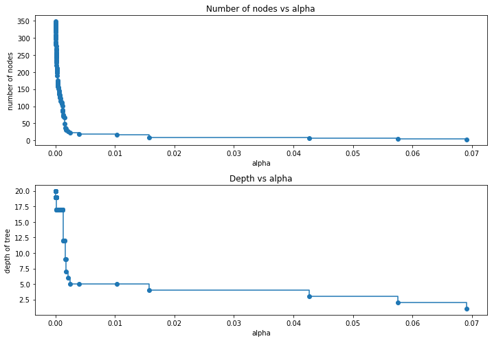
For the remainder, we remove the last element in clfs and ccp_alphas, because it is the trivial tree with only one node. Here we show that the number of nodes and tree depth decreases as alpha increases.

In [ ]:

clfs = clfs[:-1]
ccp_alphas = ccp_alphas[:-1]

node_counts = [clf.tree_.node_count for clf in clfs]
depth = [clf.tree_.max_depth for clf in clfs]
fig, ax = plt.subplots(2, 1, figsize=(10, 7))
ax[0].plot(ccp_alphas, node_counts, marker="o", drawstyle="steps-post")
ax[0].set_xlabel("alpha")
ax[0].set_ylabel("number of nodes")
ax[0].set_title("Number of nodes vs alpha")
ax[1].plot(ccp_alphas, depth, marker="o", drawstyle="steps-post")
ax[1].set_xlabel("alpha")
ax[1].set_ylabel("depth of tree")
ax[1].set_title("Depth vs alpha")
fig.tight_layout()

In [ ]:

recall_train = []
for clf in clfs:
    pred_train = clf.predict(X_train)
    values_train = recall_score(y_train, pred_train)
    recall_train.append(values_train)

In [ ]:

recall_test = []
for clf in clfs:
    pred_test = clf.predict(X_test)
    values_test = recall_score(y_test, pred_test)
    recall_test.append(values_test)

In [ ]:

train_scores = [clf.score(X_train, y_train) for clf in clfs]
test_scores = [clf.score(X_test, y_test) for clf in clfs]

In [ ]:

fig, ax = plt.subplots(figsize=(15, 5))
ax.set_xlabel("alpha")
ax.set_ylabel("Recall")
ax.set_title("Recall vs alpha for training and testing sets")
ax.plot(
    ccp_alphas, recall_train, marker="o", label="train", drawstyle="steps-post",
)
ax.plot(ccp_alphas, recall_test, marker="o", label="test", drawstyle="steps-post")
ax.legend()
plt.show()

In [ ]:

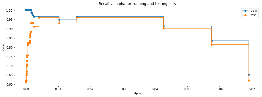
# creating the model where we get highest train and test recall
index_best_model = np.argmax(recall_test)
best_model = clfs[index_best_model]
print(best_model)

DecisionTreeClassifier(ccp_alpha=0.004008680486241742, class_weight='balanced',
                       random_state=1)

In [ ]:

confusion_matrix_sklearn(best_model, X_train, y_train)

In [ ]:

decision_tree_post_perf_train = model_performance_classification_sklearn(
    best_model, X_train, y_train
)
decision_tree_post_perf_train

Out[ ]:

	Accuracy	Recall	Precision	F1
0	0.91143	0.96610	0.27143	0.42379

In [ ]:

confusion_matrix_sklearn(best_model, X_test, y_test)

In [ ]:

decision_tree_post_test = model_performance_classification_sklearn(
    best_model, X_test, y_test
)
decision_tree_post_test

Out[ ]:

	Accuracy	Recall	Precision	F1
0	0.91733	0.96117	0.28863	0.44395

In the post-pruned tree also, the model is giving a generalized result since the recall scores on both the train and test data are coming to be around 0.96 which shows that the model is able to generalize well on unseen data.

In [ ]:

plt.figure(figsize=(20, 10))

out = tree.plot_tree(
    best_model,
    feature_names=feature_names,
    filled=True,
    fontsize=9,
    node_ids=False,
    class_names=None,
)
for o in out:
    arrow = o.arrow_patch
    if arrow is not None:
        arrow.set_edgecolor("black")
        arrow.set_linewidth(1)
plt.show()

In [ ]:

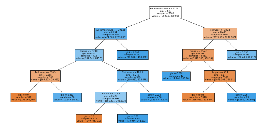
# Text report showing the rules of a decision tree -

print(tree.export_text(best_model, feature_names=feature_names, show_weights=True))

|--- Rotational speed <= 1379.50
|   |--- Air temperature <= 301.55
|   |   |--- Torque <= 52.85
|   |   |   |--- Tool wear <= 206.50
|   |   |   |   |--- weights: [176.97, 0.00] class: 0
|   |   |   |--- Tool wear >  206.50
|   |   |   |   |--- weights: [10.35, 59.32] class: 1
|   |   |--- Torque >  52.85
|   |   |   |--- Tool wear <= 185.50
|   |   |   |   |--- Torque <= 62.35
|   |   |   |   |   |--- weights: [140.75, 0.00] class: 0
|   |   |   |   |--- Torque >  62.35
|   |   |   |   |   |--- weights: [10.87, 341.10] class: 1
|   |   |   |--- Tool wear >  185.50
|   |   |   |   |--- weights: [9.31, 474.58] class: 1
|   |--- Air temperature >  301.55
|   |   |--- weights: [76.06, 1408.90] class: 1
|--- Rotational speed >  1379.50
|   |--- Tool wear <= 202.50
|   |   |--- Torque <= 15.45
|   |   |   |--- weights: [11.90, 281.78] class: 1
|   |   |--- Torque >  15.45
|   |   |   |--- Torque <= 58.40
|   |   |   |   |--- weights: [2865.61, 118.64] class: 0
|   |   |   |--- Torque >  58.40
|   |   |   |   |--- weights: [5.69, 177.97] class: 1
|   |--- Tool wear >  202.50
|   |   |--- weights: [192.49, 637.71] class: 1

We can see that the observation we got from the pre-pruned tree is also matching with the decision tree rules of the post pruned tree.

In [ ]:

importances = best_model.feature_importances_
indices = np.argsort(importances)

In [ ]:

plt.figure(figsize=(12, 12))
plt.title("Feature Importances")
plt.barh(range(len(indices)), importances[indices], color="violet", align="center")
plt.yticks(range(len(indices)), [feature_names[i] for i in indices])
plt.xlabel("Relative Importance")
plt.show()

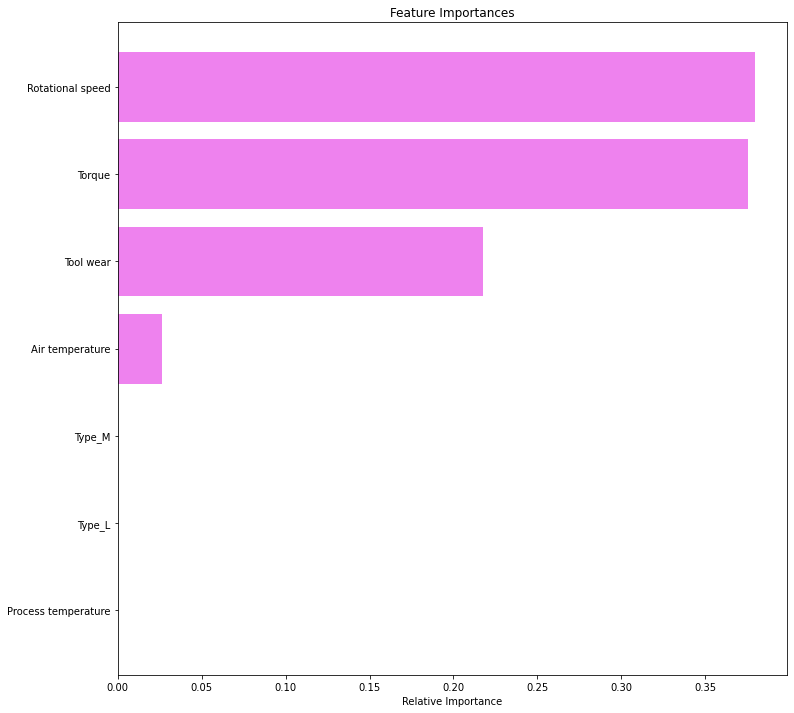
Rotational speed and Torque are the most important features for the post pruned tree

Comparison of Models and Final Model Selection

In [ ]:

# training performance comparison

models_train_comp_df = pd.concat(
    [
        decision_tree_perf_train_without.T,
        decision_tree_perf_train.T,
        decision_tree_tune_perf_train.T,
        decision_tree_post_perf_train.T,
    ],
    axis=1,
)
models_train_comp_df.columns = [
    "Decision Tree without class_weight",
    "Decision Tree with class_weight",
    "Decision Tree (Pre-Pruning)",
    "Decision Tree (Post-Pruning)",
]
print("Training performance comparison:")
models_train_comp_df

Training performance comparison:

Out[ ]:

	Decision Tree without class_weight	Decision Tree with class_weight	Decision Tree (Pre-Pruning)	Decision Tree (Post-Pruning)
Accuracy	1.00000	1.00000	0.87343	0.91143
Recall	1.00000	1.00000	0.96610	0.96610
Precision	1.00000	1.00000	0.20615	0.27143
F1	1.00000	1.00000	0.33979	0.42379

In [ ]:

# testing performance comparison

models_test_comp_df = pd.concat(
    [
        decision_tree_perf_test_without.T,
        decision_tree_perf_test.T,
        decision_tree_tune_perf_test.T,
        decision_tree_post_test.T,
    ],
    axis=1,
)
models_test_comp_df.columns = [
    "Decision Tree without class_weight",
    "Decision Tree with class_weight",
    "Decision Tree (Pre-Pruning)",
    "Decision Tree (Post-Pruning)",
]
print("Test set performance comparison:")
models_test_comp_df

Test set performance comparison:

Out[ ]:

	Decision Tree without class_weight	Decision Tree with class_weight	Decision Tree (Pre-Pruning)	Decision Tree (Post-Pruning)
Accuracy	0.97567	0.97700	0.88167	0.91733
Recall	0.72816	0.61165	0.96117	0.96117
Precision	0.62500	0.68478	0.22000	0.28863
F1	0.67265	0.64615	0.35805	0.44395

Decision tree models with pre-pruning and post-pruning both are giving equally high recall scores on both training and test sets.
However, we will choose the post pruned tree as the best model since it is giving a slightly high precision score on the train and test sets than the pre-pruned tree.

Conclusions and Recommendations

The model built can be used to predict if a machine is going to fail or not and can correctly identify 96.1% of the machine failures
Rotational speed, torque and tool wear are the most important variables in predicting whether a machine will fail or not

From the decision tree, it has been observed that if the rotational speed is less than or equal to 1379.50, the air temperature is less than or equal to 301.55, the torque is less than or equal to 52.85 and the tool wear is greater than 206.50, then the machine is most likey to fail
- The company should give a vigilant eye for these values in order to detect machine failure.
The company should use more data for the analysis to get more reliable results
As the variable used vary with the type of operation (turning, drilling, etc.) being performed, the company can look to build separate models for each different type of operation

Appendix: Detailed Exploratory Data Analysis (EDA)

Univariate Analysis

Observation on Air temperature

In [ ]:

histogram_boxplot(data, "Air temperature")

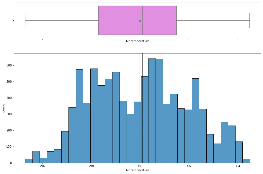
The air temperature distribution looks slightly left skewed with a mean temperature around 300K.
There is no outlier present.

Observation on Process temperature

In [ ]:

histogram_boxplot(data, "Process temperature")

The process temperature distribution looks slightly left skewed with a mean temperature around 329K.
There is no outlier present.

Observation on Rotational Speed

In [ ]:

histogram_boxplot(data, "Rotational speed")

The rotational speed is right skewed with many outliers on the upper quartile.
Some of the manufacturing operations are performed at a higher speed.

Observation on Torque

In [ ]:

histogram_boxplot(data, "Torque")

The distribution of torque is normal with mean torque around 40 Nm.
Outliers are present on both sides.

Observation on Tool Wear

In [ ]:

histogram_boxplot(data, "Tool wear")

Tool wear is uniformly distributed with some of the higher values being less frequent.

Observation on Type of product

In [ ]:

labeled_barplot(data, "Type", perc=True)

Around 60% of products are of low quality, 30% are of medium quality whereas 10% are of high quality

Observation on `Failure`

In [ ]:

labeled_barplot(data, "Failure", perc=True)

In 96.6% of observations the machine does not fail while in 3.4% of observations it fails.

Bivariate Analysis

Correlation Check

In [ ]:

cols_list = data.select_dtypes(include=np.number).columns.tolist()
cols_list.remove('Failure')

plt.figure(figsize=(12, 7))
sns.heatmap(
    data[cols_list].corr(), annot=True, vmin=-1, vmax=1, fmt=".2f", cmap="Spectral"
)
plt.show()

There’s a positive correlation between the air temperature and process temperature.
There’s a negative correlation between the rotational speed and torque.
No other variables are correlated. We will analyze it further.

Observation on `Type` vs `Air temperature`

In [ ]:

plt.figure(figsize=(10, 5))
sns.boxplot(data=data, x="Type", y="Air temperature")
plt.show()

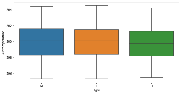
There is no distinct difference in values of Air temperature and Type

Observation on `Type` vs `Process temperature`

In [ ]:

plt.figure(figsize=(10, 5))
sns.boxplot(data=data, x="Type", y="Process temperature")
plt.show()

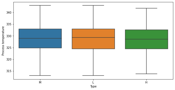
There is no distinct difference in values of Process temperature and Type for M and L types.
Lesser Process temperature is observed in manufacturing H type of products.

Observation on `Type` vs `Rotational speed`

In [ ]:

plt.figure(figsize=(10, 5))
sns.boxplot(data=data, x="Type", y="Rotational speed")
plt.show()

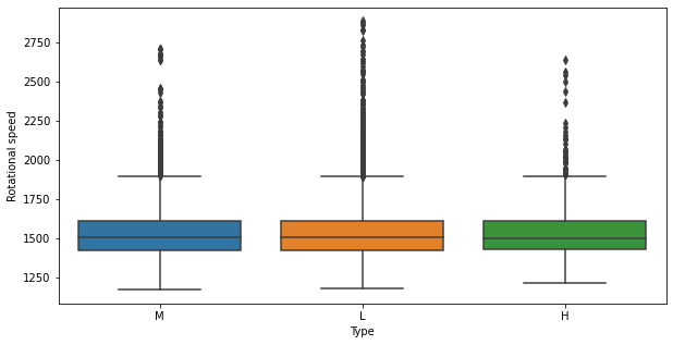
Some of the L type of products are manufactured at higher rotational speed

Observation on `Type` vs `Tool wear`

In [ ]:

plt.figure(figsize=(10, 5))
sns.boxplot(data=data, x="Type", y="Tool wear")
plt.show()

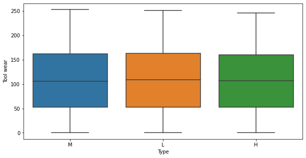
There is no distinct difference in values of Tool wear and Type

Observation on `Type` vs `Torque`

In [ ]:

plt.figure(figsize=(10, 5))
sns.boxplot(data=data, x="Type", y="Torque")
plt.show()

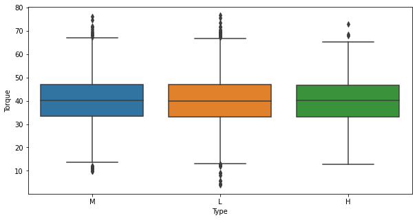
Some of the L type products are manufactured at lower Toque as compared to M and H type of products.

Failure vs Type

Let’s see how the target variable varies across the type of the product

In [ ]:

stacked_barplot(data, "Type", "Failure")

Failure     0    1    All
Type                     
All      9661  339  10000
L        5765  235   6000
M        2914   83   2997
H         982   21   1003
------------------------------------------------------------------------------------------------------------------------

Around 70 % of the failure occurred during machining of L type i.e., low-quality products.
Machining of high-quality products is less prone to failure.

Distribution of numerical input variables by failure status

Let’s analyze the relation between Air temperature and Failure.

In [ ]:

distribution_plot_wrt_target(data, "Air temperature", "Failure")

Most of the failures of the manufacturing system occur at higher Air temperature.

Let’s analyze the relation between Process temperature and Failure.

In [ ]:

distribution_plot_wrt_target(data, "Process temperature", "Failure")

Most of the failures of the manufacturing system occur at higher Process temperature.

Let’s analyze the relation between Rotational speed and Failure.

In [ ]:

distribution_plot_wrt_target(data, "Rotational speed", "Failure")

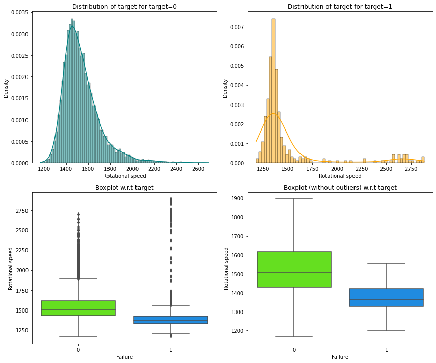
Manufacturing system is more prone to failure at lower Rotational speed than at higher rotational speed.

Let’s analyze the relation between Torque and Failure.

In [ ]:

distribution_plot_wrt_target(data, "Torque", "Failure")

Most of the failures of the manufacturing system occur at higher torque as compared to lower values of torque.

Let’s analyze the relation between Tool wear and Failure.

In [ ]:

distribution_plot_wrt_target(data, "Tool wear", "Failure")

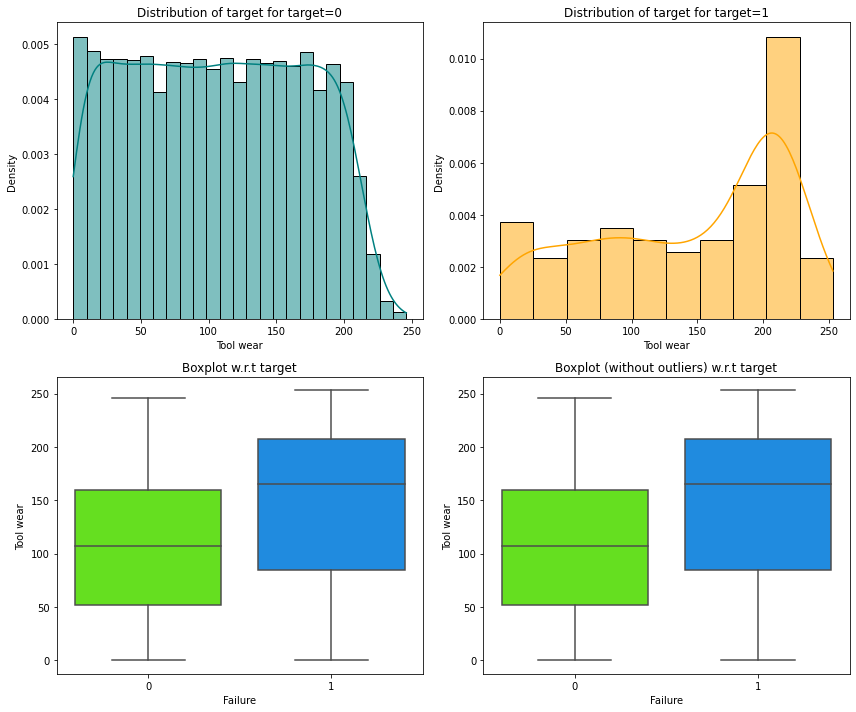
Most of the failures occur at higher values of tool wear than at lower tool wear.

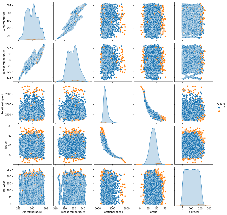
In [ ]:

sns.pairplot(data, hue="Failure")

Out[ ]:

<seaborn.axisgrid.PairGrid at 0x7f68dcb4ac10>

The correlation between air temperature and process temperature and torque and rotational speed is visible here too

Creating Decision Trees for Classification Problems - Machine Failure Prediction

Creating Decision Trees for Classification Problems – Machine Failure Prediction

Problem Statement

Business Context

Objective

Dataset

Data Description

Importing the necessary libraries

Loading the dataset

Overview of the dataset

View the first and last 5 rows of the dataset.

Understand the shape of the dataset.

Check the data types of the columns for the dataset.

Checking for missing values

Dropping the duplicate values

Dropping the columns with all unique values

Statistical summary of the data

Exploratory Data Analysis (EDA) Summary

Note: The EDA section has been covered multiple times in the previous case studies. In this case study, we will mainly focus on the model building aspects. We will only be looking at the key observations from EDA. The detailed EDA can be found in the appendix section.

Univariate Analysis

Bivariate Analysis

Data Preprocessing

Outlier Detection

Data Preparation for Modeling

Model Building

Decision Tree (default)

Model Evaluation

Decision Tree (with class_weights)

Decision Tree (Pre-pruning)

Decision Tree (Post pruning)

Comparison of Models and Final Model Selection

Conclusions and Recommendations

Appendix: Detailed Exploratory Data Analysis (EDA)

Univariate Analysis

Observation on Air temperature

Observation on Process temperature

Observation on Rotational Speed

Observation on Torque

Observation on Tool Wear

Observation on Type of product

Observation on Failure

Bivariate Analysis

Correlation Check

Observation on Type vs Air temperature

Observation on Type vs Process temperature

Observation on Type vs Rotational speed

Observation on Type vs Tool wear

Observation on Type vs Torque

Failure vs Type

Distribution of numerical input variables by failure status

Leave a Reply Cancel reply

Observation on `Failure`

Observation on `Type` vs `Air temperature`

Observation on `Type` vs `Process temperature`

Observation on `Type` vs `Rotational speed`

Observation on `Type` vs `Tool wear`

Observation on `Type` vs `Torque`