General Middleware
Predicting Classification Models
Case Study: German Credit Analysis
Context:
To minimize loss from the bank’s perspective, the bank needs a decision rule regarding whom to approve the loan and whom not to. An applicant’s demographic and socio-economic profiles are considered by loan managers before a decision is taken regarding his/her loan application.
In this dataset, each entry represents a person who takes credit from a bank. Each person is classified as a good or bad credit risk according to the set of attributes.
Objective:
The objective is to build a predictive model on this data to help the bank take a decision on whether to approve a loan to a prospective applicant.
Attribute Information:
- The data contains characteristics of the people
- Age (Numeric: Age in years)
- Sex (Categories: male, female)
- Job (Categories: unskilled and non-resident, unskilled and resident, skilled, highly skilled)
- Housing (Categories: own, rent, or free)
- Saving accounts (Categories: little, moderate, quite rich, rich)
- Checking account (Categories: little, moderate, rich)
- Credit amount (Numeric: Amount of credit in DM – Deutsche Mark)
- Duration (Numeric: Duration for which the credit is given in months)
- Purpose (Categories: car, furniture/equipment, radio/TV, domestic appliances, repairs, education, business, vacation/others)
- Risk (0 – Person is not at risk, 1 – Person is at risk(defaulter))
Learning Outcomes:
- Exploratory Data Analysis
- Preparing the data to train a model
- Training and understanding of data using a logistic regression model
- Model evaluation
Steps and Tasks:
- Import Libraries and Load Dataset
- Overview of data
- Data Visualization
- Data preparation
- Choose Model, Train, and Evaluate
- Conclusion
Dataset:
Solution Jupyter Notebook:
Let’s start by importing necessary libraries
In [1]:
# this will help in making the Python code more structured automatically (good coding practice)
%load_ext nb_black

import warnings

warnings.filterwarnings("ignore")

# Libraries to help with reading and manipulating data

import pandas as pd
import numpy as np

# Library to split data
from sklearn.model_selection import train_test_split

# libaries to help with data visualization
import matplotlib.pyplot as plt
import seaborn as sns

# Removes the limit for the number of displayed columns
pd.set_option("display.max_columns", None)
# Sets the limit for the number of displayed rows
pd.set_option("display.max_rows", 200)


# To build model for prediction

from sklearn.linear_model import LogisticRegression

# To get diferent metric scores
# To get diferent metric scores

from sklearn.metrics import (
    f1_score,
    accuracy_score,
    recall_score,
    precision_score,
    confusion_matrix,
    roc_auc_score,
    plot_confusion_matrix,
    precision_recall_curve,
    roc_curve,
)
Load and overview the dataset
In [2]:
# Loading the dataset - sheet_name parameter is used if there are multiple tabs in the excel file.
data = pd.read_csv("German_Credit.csv")
In [3]:
data.head()
Out[3]:
| Age | Sex | Job | Housing | Saving accounts | Checking account | Credit amount | Duration | Risk | Purpose | |
|---|---|---|---|---|---|---|---|---|---|---|
| 0 | 67 | male | skilled | own | little | little | 1169 | 6 | 0 | radio/TV |
| 1 | 22 | female | skilled | own | little | moderate | 5951 | 48 | 1 | radio/TV |
| 2 | 49 | male | unskilled_and_non-resident | own | little | little | 2096 | 12 | 0 | education |
| 3 | 45 | male | skilled | free | little | little | 7882 | 42 | 0 | furniture/equipment |
| 4 | 53 | male | skilled | free | little | little | 4870 | 24 | 1 | car |
Understand the shape of the dataset.
In [4]:
data.shape
Out[4]:
(1000, 10)
Check the data types of the columns in the dataset.
In [5]:
data.info()
<class 'pandas.core.frame.DataFrame'>
RangeIndex: 1000 entries, 0 to 999
Data columns (total 10 columns):
 #   Column            Non-Null Count  Dtype
---  ------            --------------  -----
 0   Age               1000 non-null   int64
 1   Sex               1000 non-null   object
 2   Job               1000 non-null   object
 3   Housing           1000 non-null   object
 4   Saving accounts   1000 non-null   object
 5   Checking account  1000 non-null   object
 6   Credit amount     1000 non-null   int64
 7   Duration          1000 non-null   int64
 8   Risk              1000 non-null   int64
 9   Purpose           1000 non-null   object
dtypes: int64(4), object(6)
memory usage: 78.2+ KB
- There are total 10 columns and 1,000 observations in the dataset
- We have only three continuous variables – Age, Credit Amount, and Duration.
- All other variables are categorical.
- There no missing values in the dataset.
Summary of the data
In [6]:
data.describe().T
Out[6]:
| count | mean | std | min | 25% | 50% | 75% | max | |
|---|---|---|---|---|---|---|---|---|
| Age | 1000.0 | 35.546 | 11.375469 | 19.0 | 27.0 | 33.0 | 42.00 | 75.0 |
| Credit amount | 1000.0 | 3271.258 | 2822.736876 | 250.0 | 1365.5 | 2319.5 | 3972.25 | 18424.0 |
| Duration | 1000.0 | 20.903 | 12.058814 | 4.0 | 12.0 | 18.0 | 24.00 | 72.0 |
| Risk | 1000.0 | 0.300 | 0.458487 | 0.0 | 0.0 | 0.0 | 1.00 | 1.0 |
Observations
- Mean value for the age column is approx 35 and the median is 33. This shows that majority of the customers are under 35 years of age.
- Mean amount of credit is approx 3,271 but it has a wide range with values from 250 to 18,424. We will explore this further in univariate analysis.
- Mean duration for which the credit is given is approx 21 months.
In [7]:
# Making a list of all catrgorical variables
cat_col = [
    "Sex",
    "Job",
    "Housing",
    "Saving accounts",
    "Checking account",
    "Purpose",
    "Risk",
]

# Printing number of count of each unique value in each column
for column in cat_col:
    print(data[column].value_counts())
    print("-" * 40)
male      690
female    310
Name: Sex, dtype: int64
----------------------------------------
skilled                       630
unskilled_and_non-resident    222
highly skilled                148
Name: Job, dtype: int64
----------------------------------------
own     713
rent    179
free    108
Name: Housing, dtype: int64
----------------------------------------
little        786
moderate      103
quite rich     63
rich           48
Name: Saving accounts, dtype: int64
----------------------------------------
moderate    472
little      465
rich         63
Name: Checking account, dtype: int64
----------------------------------------
car                    337
radio/TV               280
furniture/equipment    181
business                97
education               59
repairs                 22
domestic appliances     12
vacation/others         12
Name: Purpose, dtype: int64
----------------------------------------
0    700
1    300
Name: Risk, dtype: int64
----------------------------------------
- We have more male customers as compared to female customers
- There are very few observations i.e., only 22 for customers with job category – unskilled and non-resident
- We can see that the distribution of classes in the target variable is imbalanced i.e., only 30% observations with defaulters.
- Most of the customers are not at risk.
Univariate analysis
In [8]:
def histogram_boxplot(data, feature, figsize=(12, 7), kde=False, bins=None):
    """
    Boxplot and histogram combined

    data: dataframe
    feature: dataframe column
    figsize: size of figure (default (12,7))
    kde: whether to show the density curve (default False)
    bins: number of bins for histogram (default None)
    """
    f2, (ax_box2, ax_hist2) = plt.subplots(
        nrows=2,  # Number of rows of the subplot grid= 2
        sharex=True,  # x-axis will be shared among all subplots
        gridspec_kw={"height_ratios": (0.25, 0.75)},
        figsize=figsize,
    )  # creating the 2 subplots
    sns.boxplot(
        data=data, x=feature, ax=ax_box2, showmeans=True, color="violet"
    )  # boxplot will be created and a star will indicate the mean value of the column
    sns.histplot(
        data=data, x=feature, kde=kde, ax=ax_hist2, bins=bins, palette="winter"
    ) if bins else sns.histplot(
        data=data, x=feature, kde=kde, ax=ax_hist2
    )  # For histogram
    ax_hist2.axvline(
        data[feature].mean(), color="green", linestyle="--"
    )  # Add mean to the histogram
    ax_hist2.axvline(
        data[feature].median(), color="black", linestyle="-"
    )  # Add median to the histogram
Observation on Age
In [9]:
histogram_boxplot(data, "Age")
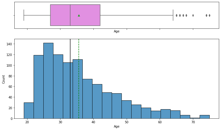
- The distribution of age is right-skewed
- The boxplot shows that there are outliers at the right end
- We will not treat these outliers as they represent the real market trend
Observation on Credit Amount
In [10]:
histogram_boxplot(data, "Credit amount")
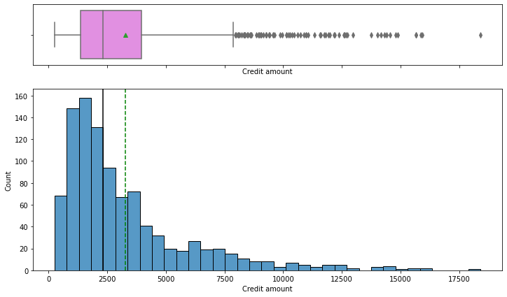
- The distribution of the credit amount is right-skewed
- The boxplot shows that there are outliers at the right end
- We will not treat these outliers as they represent the real market trend
Observations on Duration
In [11]:
histogram_boxplot(data, "Duration")
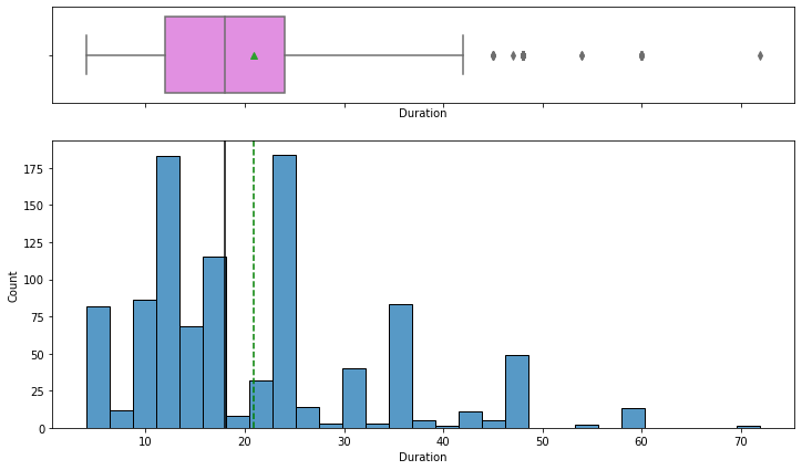
- The distribution of the duration for which the credit is given is right-skewed
- The boxplot shows that there are outliers at the right end
- We will not treat these outliers as they represent the real market trend
In [12]:
# function to create labeled barplots


def labeled_barplot(data, feature, perc=False, n=None):
    """
    Barplot with percentage at the top

    data: dataframe
    feature: dataframe column
    perc: whether to display percentages instead of count (default is False)
    n: displays the top n category levels (default is None, i.e., display all levels)
    """

    total = len(data[feature])  # length of the column
    count = data[feature].nunique()
    if n is None:
        plt.figure(figsize=(count + 1, 5))
    else:
        plt.figure(figsize=(n + 1, 5))

    plt.xticks(rotation=90, fontsize=15)
    ax = sns.countplot(
        data=data,
        x=feature,
        palette="Paired",
        order=data[feature].value_counts().index[:n].sort_values(),
    )

    for p in ax.patches:
        if perc == True:
            label = "{:.1f}%".format(
                100 * p.get_height() / total
            )  # percentage of each class of the category
        else:
            label = p.get_height()  # count of each level of the category

        x = p.get_x() + p.get_width() / 2  # width of the plot
        y = p.get_height()  # height of the plot

        ax.annotate(
            label,
            (x, y),
            ha="center",
            va="center",
            size=12,
            xytext=(0, 5),
            textcoords="offset points",
        )  # annotate the percentage

    plt.show()  # show the plot
Observations on Risk
In [13]:
labeled_barplot(data, "Risk", perc=True)
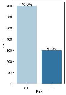
- As mentioned earlier, the class distribution in the target variable is imbalanced.
- We have 70% observations for non-defaulters and 30% observations for defaulters.
Observations on Sex of Customers
In [14]:
labeled_barplot(data, "Sex", perc=True)
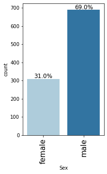
- Male customers are taking more credit than female customers
- There are 69% male customers and 31% female customers
Observations on Housing
In [15]:
labeled_barplot(data, "Housing", perc=True)
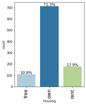
- Major of the customers, approx 71%, who take credit have their own house
- Approx 18% customers are living in a rented house
- There are only 11% customers who have free housing. These are the customers who live in a house given by their company or organization
Observations on Job
In [16]:
labeled_barplot(data, "Job", perc=True)

- Majority of the customers i.e. 63% fall into the skilled category.
- There are only approx 15% customers that lie in highly skilled category which makes sense as these may be the persons with high education or highly experienced.
- There are very few observations, approx 22%, with 0 or 1 job category.
Observations on Saving accounts
In [17]:
labeled_barplot(data, "Saving accounts", perc=True)
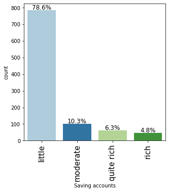
- Approx 70% customers who take credit have a little or moderate amount in their savings account. This makes sense as these customers would need credit more than the other categories.
- Approx 11% customers who take credit are in the rich category based on their balance in the savings account.
- Note that the percentages do not add up to 100 as we have missing values in this column.
Observations on Checking account
In [18]:
labeled_barplot(data, "Checking account", perc=True)
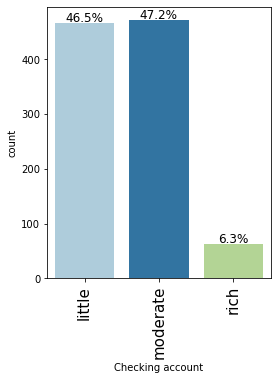
- Approx 54% customers who take credit have a little or moderate amount in their checking account. This makes sense as these customers would need credit more than the other categories.
- Approx 6% customers who take credit are in the rich category based on their balance in the checking account.
- Note that the percentages do not add up to 100 as we have missing values in this column.
Observations on Purpose
In [19]:
labeled_barplot(data, "Purpose", perc=True)
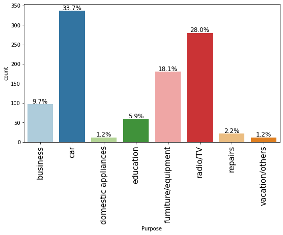
- The plot shows that most customers take credit for luxury items like car, radio or furniture/equipment, domestic appliances.
- Approximately just 16% customers take credit for business or education
Bivariate Analysis
In [20]:
sns.pairplot(data, hue="Risk")
plt.show()
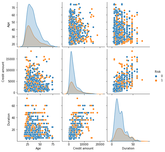
- There are overlaps i.e., no clear distinction in the distribution of variables for people who have defaulted and did not default.
- Let’s explore this further with the help of other plots.
In [21]:
### function to plot distributions wrt target


def distribution_plot_wrt_target(data, predictor, target):

    fig, axs = plt.subplots(2, 2, figsize=(12, 10))

    target_uniq = data[target].unique()

    axs[0, 0].set_title("Distribution of target for target=" + str(target_uniq[0]))
    sns.histplot(
        data=data[data[target] == target_uniq[0]],
        x=predictor,
        kde=True,
        ax=axs[0, 0],
        color="teal",
        stat="density",
    )

    axs[0, 1].set_title("Distribution of target for target=" + str(target_uniq[1]))
    sns.histplot(
        data=data[data[target] == target_uniq[1]],
        x=predictor,
        kde=True,
        ax=axs[0, 1],
        color="orange",
        stat="density",
    )

    axs[1, 0].set_title("Boxplot w.r.t target")
    sns.boxplot(data=data, x=target, y=predictor, ax=axs[1, 0], palette="gist_rainbow")

    axs[1, 1].set_title("Boxplot (without outliers) w.r.t target")
    sns.boxplot(
        data=data,
        x=target,
        y=predictor,
        ax=axs[1, 1],
        showfliers=False,
        palette="gist_rainbow",
    )

    plt.tight_layout()
    plt.show()
Risk vs Age
In [22]:
distribution_plot_wrt_target(data, "Age", "Risk")
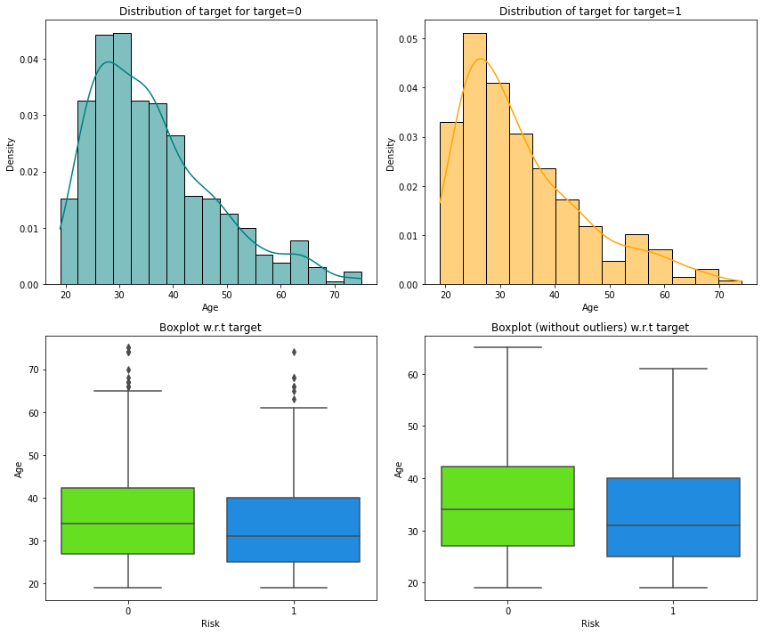
- We can see that the median age of defaulters is less than the median age of non-defaulters.
- This shows that younger customers are more likely to default.
- There are outliers in boxplots of both class distributions
Risk vs Credit amount
In [23]:
distribution_plot_wrt_target(data, "Credit amount", "Risk")
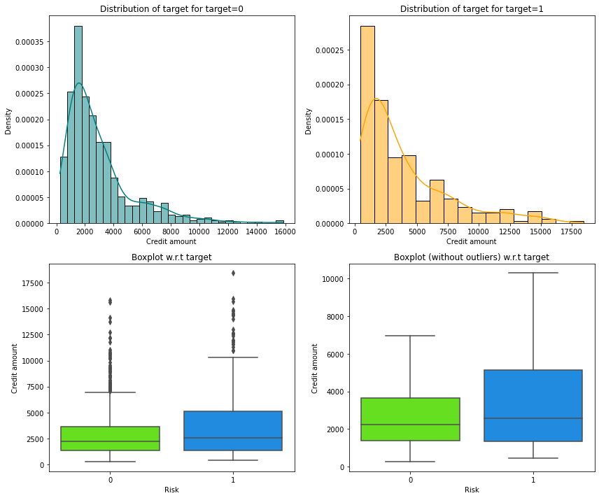
- We can see that the third quartile amount of defaulters is much more than the third quartile amount of non-defaulters.
- This shows that customers with high credit amount are more likely to default.
- There are outliers in boxplots of both class distributions
Risk vs Duration
In [24]:
distribution_plot_wrt_target(data, "Duration", "Risk")

- We can see that the second and third quartiles of duration of defaulters is much more than the second and third quartiles duration of non-defaulters.
- This shows that customers with high duration are more likely to default.
Risk vs Saving accounts
In [25]:
distribution_plot_wrt_target(data, "Age", "Saving accounts")
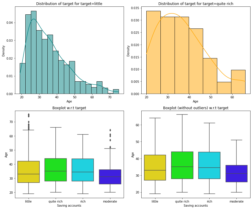
- The plot shows that customers with higher age are in the rich or quite rich categories.
- Age of the customers in the little and moderate categories is slightly less but there are outliers in both of the distributions.
In [26]:
# function to plot stacked bar chart


def stacked_barplot(data, predictor, target):
    """
    Print the category counts and plot a stacked bar chart

    data: dataframe
    predictor: independent variable
    target: target variable
    """
    count = data[predictor].nunique()
    sorter = data[target].value_counts().index[-1]
    tab1 = pd.crosstab(data[predictor], data[target], margins=True).sort_values(
        by=sorter, ascending=False
    )
    print(tab1)
    print("-" * 120)
    tab = pd.crosstab(data[predictor], data[target], normalize="index").sort_values(
        by=sorter, ascending=False
    )
    tab.plot(kind="bar", stacked=True, figsize=(count + 5, 6))
    plt.legend(
        loc="lower left", frameon=False,
    )
    plt.legend(loc="upper left", bbox_to_anchor=(1, 1))
    plt.show()
Risk vs Sex
In [27]:
stacked_barplot(data, "Sex", "Risk")
Risk      0    1   All
Sex
All     700  300  1000
male    499  191   690
female  201  109   310
------------------------------------------------------------------------------------------------------------------------
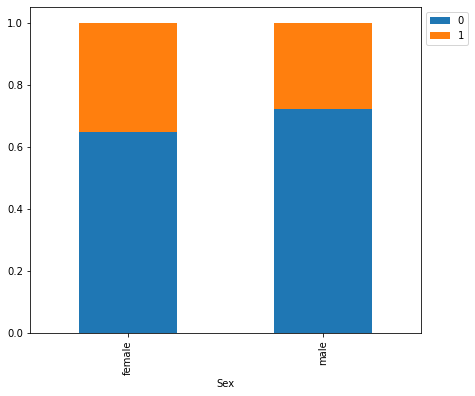
- We saw earlier that the percentage of male customers is more than the female customers. This plot shows that female customers are more likely to default as compared to male customers.
Risk vs Job
In [28]:
stacked_barplot(data, "Job", "Risk")
Risk                          0    1   All
Job
All                         700  300  1000
skilled                     444  186   630
unskilled_and_non-resident  159   63   222
highly skilled               97   51   148
------------------------------------------------------------------------------------------------------------------------
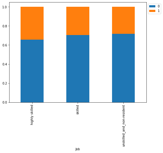
- There are no significant difference with respect to the job level
- However, highly skilled or unskilled/non-resident customers are more likely to default as compared to customers in 1 or 2 category
Risk vs Housing
In [29]:
stacked_barplot(data, "Housing", "Risk")
Risk       0    1   All
Housing
All      700  300  1000
own      527  186   713
rent     109   70   179
free      64   44   108
------------------------------------------------------------------------------------------------------------------------
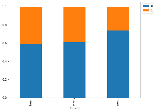
- Customers owning a house are less likely to default
- Customers with free or rented housing are almost at same risk of default
Risk vs Saving accounts
In [30]:
stacked_barplot(data, "Saving accounts", "Risk")
Risk               0    1   All
Saving accounts
All              700  300  1000
little           537  249   786
moderate          69   34   103
quite rich        52   11    63
rich              42    6    48
------------------------------------------------------------------------------------------------------------------------
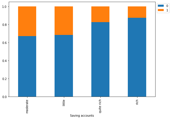
- As we saw earlier, customers with little or moderate amounts in saving accounts takes more credit but at the same time they are most likely to default.
- Rich customers are slightly less likely to default as compared to quite rich customers
Risk vs Checking account
In [31]:
stacked_barplot(data, "Checking account", "Risk")
Risk                0    1   All
Checking account
All               700  300  1000
little            304  161   465
moderate          347  125   472
rich               49   14    63
------------------------------------------------------------------------------------------------------------------------
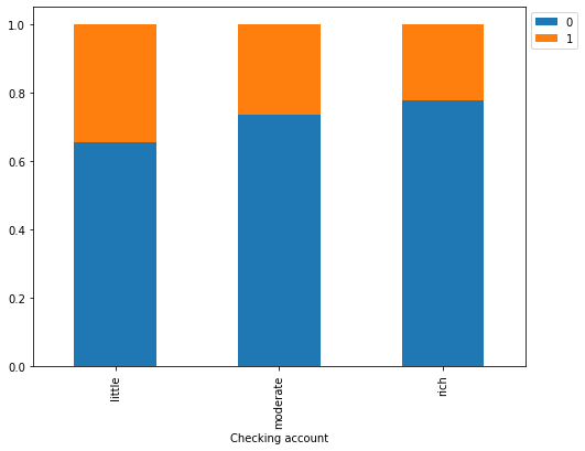
- The plot further confirms the findings of the previous plot.
- Customers with little amount in checking accounts are most likely to default as compared to customers with moderate amount, which in turn, are more likely as compared to the rich customers.
Risk vs Purpose
In [32]:
stacked_barplot(data, "Purpose", "Risk")
Risk                   0    1   All
Purpose
All                  700  300  1000
car                  231  106   337
radio/TV             218   62   280
furniture/equipment  123   58   181
business              63   34    97
education             36   23    59
repairs               14    8    22
vacation/others        7    5    12
domestic appliances    8    4    12
------------------------------------------------------------------------------------------------------------------------
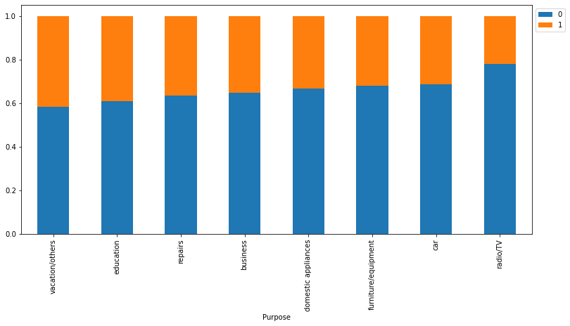
- Customers who take credit for radio/TV are least likely to default. This might be because their credit amount is small.
- Customers who take credit for education or vacation are most likely to default.
- Other categories have no significant difference between their default and non-default ratio.
In [33]:
plt.figure(figsize=(15, 7))
sns.heatmap(data.corr(), annot=True, vmin=-1, vmax=1, fmt=".2f", cmap="Spectral")
plt.show()
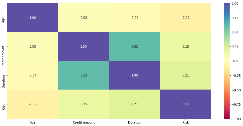
- Credit amount and duration have positive correlation which makes sense as customers might take the credit for longer duration if the amount of credit is high.
- Other variables have no significant correlation between them.
Model evaluation criterion
Model can make wrong predictions as:
- Predicting a customer is not going to default but in reality the customer will default – Loss of resources (FN)
- Predicting a customer is going to default but in reality the customer will not default – Loss of opportunity (FP)
Which Loss is greater ?
- Loss of resources will be the greater loss as the bank will be losing on its resources/money.
How to reduce this loss i.e need to reduce False Negatives ?
- Company would want to reduce false negatives, this can be done by maximizing the Recall. Greater the recall lesser the chances of false negatives.
First, let’s create functions to calculate different metrics and confusion matrix so that we don’t have to use the same code repeatedly for each model.
- The model_performance_classification_sklearn_with_threshold function will be used to check the model performance of models.
- The confusion_matrix_sklearn_with_threshold function will be used to plot confusion matrix.
In [34]:
# defining a function to compute different metrics to check performance of a classification model built using sklearn

def model_performance_classification_sklearn_with_threshold(model, predictors, target, threshold=0.5):
    """
    Function to compute different metrics, based on the threshold specified, to check classification model performance

    model: classifier
    predictors: independent variables
    target: dependent variable
    threshold: threshold for classifying the observation as class 1
    """

    # predicting using the independent variables
    pred_prob = model.predict_proba(predictors)[:, 1]
    pred_thres = pred_prob > threshold
    pred = np.round(pred_thres)

    acc = accuracy_score(target, pred)  # to compute Accuracy
    recall = recall_score(target, pred)  # to compute Recall
    precision = precision_score(target, pred)  # to compute Precision
    f1 = f1_score(target, pred)  # to compute F1-score

    # creating a dataframe of metrics
    df_perf = pd.DataFrame(
        {
            "Accuracy": acc,
            "Recall": recall,
            "Precision": precision,
            "F1": f1,
        },
        index=[0],
    )

    return df_perf
In [35]:
# defining a function to plot the confusion_matrix of a classification model built using sklearn
def confusion_matrix_sklearn_with_threshold(model, predictors, target, threshold=0.5):
    """
    To plot the confusion_matrix, based on the threshold specified, with percentages

    model: classifier
    predictors: independent variables
    target: dependent variable
    threshold: threshold for classifying the observation as class 1
    """
    pred_prob = model.predict_proba(predictors)[:, 1]
    pred_thres = pred_prob > threshold
    y_pred = np.round(pred_thres)

    cm = confusion_matrix(target, y_pred)
    labels = np.asarray(
        [
            ["{0:0.0f}".format(item) + "\n{0:.2%}".format(item / cm.flatten().sum())]
            for item in cm.flatten()
        ]
    ).reshape(2, 2)

    plt.figure(figsize=(6, 4))
    sns.heatmap(cm, annot=labels, fmt="")
    plt.ylabel("True label")
    plt.xlabel("Predicted label")
Data Preparation
In [36]:
# Converting monthly values to yearly
data["Duration"] = data["Duration"] / 12
In [37]:
X = data.drop("Risk", axis=1)
Y = data["Risk"]

# creating dummy variables
X = pd.get_dummies(X, drop_first=True)

# splitting in training and test set
X_train, X_test, y_train, y_test = train_test_split(
    X, Y, test_size=0.3, random_state=42
)
Logistic Regression
In [38]:
# There are different solvers available in Sklearn logistic regression
# The newton-cg solver is faster for high-dimensional data

model = LogisticRegression(solver="newton-cg", random_state=1)
lg = model.fit(X_train, y_train)
Finding the coefficients
In [39]:
log_odds = lg.coef_[0]
pd.DataFrame(log_odds, X_train.columns, columns=["coef"]).T
Out[39]:
| Age | Credit amount | Duration | Sex_male | Job_skilled | Job_unskilled_and_non-resident | Housing_own | Housing_rent | Saving accounts_moderate | Saving accounts_quite rich | Saving accounts_rich | Checking account_moderate | Checking account_rich | Purpose_car | Purpose_domestic appliances | Purpose_education | Purpose_furniture/equipment | Purpose_radio/TV | Purpose_repairs | Purpose_vacation/others | |
|---|---|---|---|---|---|---|---|---|---|---|---|---|---|---|---|---|---|---|---|---|
| coef | -0.034633 | 0.000025 | 0.354898 | -0.387275 | 0.009656 | 0.139326 | -0.81353 | -0.376454 | 0.008775 | -0.67143 | -0.8547 | -0.214163 | -0.304406 | -0.065784 | 0.211993 | 0.308467 | -0.395234 | -0.66456 | -0.044962 | 0.204389 |
Coefficient interpretations
- Coefficients of Duration, Credit amount and some categorical levels of Purpose and Job are positive, an increase in these will lead to an increase in chances of a customer being a defaulter.
- Coefficients of Age, Sex_male, Housing, Saving_accounts, and some categorical levels of Purpose and Job is negative, an increase in these will lead to a decrease in chances of a customer being a defaulter.
Converting coefficients to odds
- The coefficients of the logistic regression model are in terms of log(odd), to find the odds we have to take the exponential of the coefficients.
- Therefore, odds = exp(b)
- The percentage change in odds is given as odds = (exp(b) – 1) * 100
Odds from coefficients
In [40]:
# converting coefficients to odds
odds = np.exp(lg.coef_[0])

# finding the percentage change
perc_change_odds = (np.exp(lg.coef_[0]) - 1) * 100

# removing limit from number of columns to display
pd.set_option("display.max_columns", None)

# adding the odds to a dataframe
pd.DataFrame({"Odds": odds, "Change_odd%": perc_change_odds}, index=X_train.columns).T
Out[40]:
| Age | Credit amount | Duration | Sex_male | Job_skilled | Job_unskilled_and_non-resident | Housing_own | Housing_rent | Saving accounts_moderate | Saving accounts_quite rich | Saving accounts_rich | Checking account_moderate | Checking account_rich | Purpose_car | Purpose_domestic appliances | Purpose_education | Purpose_furniture/equipment | Purpose_radio/TV | Purpose_repairs | Purpose_vacation/others | |
|---|---|---|---|---|---|---|---|---|---|---|---|---|---|---|---|---|---|---|---|---|
| Odds | 0.965960 | 1.000025 | 1.426035 | 0.678904 | 1.009703 | 1.149499 | 0.443291 | 0.686291 | 1.008814 | 0.510978 | 0.425411 | 0.807217 | 0.737562 | 0.936333 | 1.236139 | 1.361336 | 0.673522 | 0.514500 | 0.956034 | 1.226775 |
| Change_odd% | -3.404032 | 0.002502 | 42.603495 | -32.109587 | 0.970264 | 14.949893 | -55.670940 | -31.370935 | 0.881353 | -48.902239 | -57.458924 | -19.278290 | -26.243843 | -6.366731 | 23.613943 | 36.133607 | -32.647772 | -48.550029 | -4.396613 | 22.677505 |
Coefficient interpretations
Age: Holding all other features constant a unit change in Age will decrease the odds of a customer being a defaulter by 0.96 times or a 3.40% decrease in the odds.Credit amount: Holding all other features constant a unit change in Credit amount will increase the odds of a customer being a defaulter by 1.00 times or a 0.003% increase in the odds.Duration: Holding all other features constant a unit change in Duration will increase the odds of a customer being a defaulter by 1.42 times or a 42.60% increase in the odds.Sex: The odds of a male customer being a defaulter 0.68 times less than a female customer or 32.1% fewer odds than female.Housing: The odds of a customer who has own house being a defaulter is 0.44 times less than the customer who lives in a house provided by his organization (Housing – free) or 55.67% fewer odds of being a defaulter. Similarly, The odds of a customer who lives in a rented place being a defaulter is 0.68 times less than the customer who lives in a house provided by his organization (Housing – free) or 31.37% fewer odds of being a defaulter. [Keeping housing_free as reference]
Interpretation for other attributes can be made similarly.
Checking model performance on training set
In [41]:
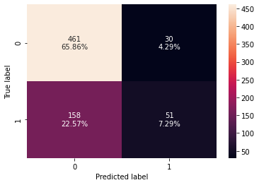
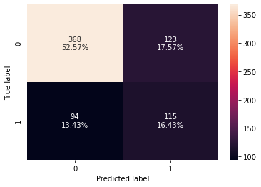
# creating confusion matrix
confusion_matrix_sklearn_with_threshold(lg, X_train, y_train)
In [42]:
log_reg_model_train_perf = model_performance_classification_sklearn_with_threshold(
    lg, X_train, y_train
)

print("Training performance:")
log_reg_model_train_perf
Training performance:
Out[42]:
| Accuracy | Recall | Precision | F1 | |
|---|---|---|---|---|
| 0 | 0.731429 | 0.244019 | 0.62963 | 0.351724 |
ROC-AUC
- ROC-AUC on training set
In [43]:
logit_roc_auc_train = roc_auc_score(y_train, lg.predict_proba(X_train)[:, 1])
fpr, tpr, thresholds = roc_curve(y_train, lg.predict_proba(X_train)[:, 1])
plt.figure(figsize=(7, 5))
plt.plot(fpr, tpr, label="Logistic Regression (area = %0.2f)" % logit_roc_auc_train)
plt.plot([0, 1], [0, 1], "r--")
plt.xlim([0.0, 1.0])
plt.ylim([0.0, 1.05])
plt.xlabel("False Positive Rate")
plt.ylabel("True Positive Rate")
plt.title("Receiver operating characteristic")
plt.legend(loc="lower right")
plt.show()
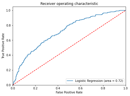
- Logistic Regression model is giving a good performance on training set but the recall is low.
Model Performance Improvement
- Let’s see if the recall score can be improved further, by changing the model threshold using AUC-ROC Curve.
Optimal threshold using AUC-ROC curve
In [44]:
# Optimal threshold as per AUC-ROC curve
# The optimal cut off would be where tpr is high and fpr is low
fpr, tpr, thresholds = roc_curve(y_train, lg.predict_proba(X_train)[:, 1])

optimal_idx = np.argmax(tpr - fpr)
optimal_threshold_auc_roc = thresholds[optimal_idx]
print(optimal_threshold_auc_roc)
0.3285584253725299
Checking model performance on training set
In [45]:
# creating confusion matrix
confusion_matrix_sklearn_with_threshold(
    lg, X_train, y_train, threshold=optimal_threshold_auc_roc
)
In [46]:
# checking model performance for this model
log_reg_model_train_perf_threshold_auc_roc = model_performance_classification_sklearn_with_threshold(
    lg, X_train, y_train, threshold=optimal_threshold_auc_roc
)
print("Training performance:")
log_reg_model_train_perf_threshold_auc_roc
Training performance:
Out[46]:
| Accuracy | Recall | Precision | F1 | |
|---|---|---|---|---|
| 0 | 0.682857 | 0.583732 | 0.474708 | 0.523605 |
- Model performance has improved significantly on training set.
- Model is giving a recall of 0.58 on the training set.
Let’s use Precision-Recall curve and see if we can find a better threshold
In [47]:
y_scores = lg.predict_proba(X_train)[:, 1]
prec, rec, tre = precision_recall_curve(y_train, y_scores,)


def plot_prec_recall_vs_tresh(precisions, recalls, thresholds):
    plt.plot(thresholds, precisions[:-1], "b--", label="precision")
    plt.plot(thresholds, recalls[:-1], "g--", label="recall")
    plt.xlabel("Threshold")
    plt.legend(loc="upper left")
    plt.ylim([0, 1])


plt.figure(figsize=(10, 7))
plot_prec_recall_vs_tresh(prec, rec, tre)
plt.show()
- At threshold around 0.37 we will get equal precision and recall but taking a step back and selecting value around 0.34 will provide a higher recall and a good precision.
In [48]:
# setting the threshold
optimal_threshold_curve = 0.34
Checking model performance on training set
In [49]:
# creating confusion matrix
confusion_matrix_sklearn_with_threshold(
    lg, X_train, y_train, threshold=optimal_threshold_curve
)
In [50]:
log_reg_model_train_perf_threshold_curve = model_performance_classification_sklearn_with_threshold(
    lg, X_train, y_train, threshold=optimal_threshold_curve
)
print("Training performance:")
log_reg_model_train_perf_threshold_curve
Training performance:
Out[50]:
| Accuracy | Recall | Precision | F1 | |
|---|---|---|---|---|
| 0 | 0.69 | 0.550239 | 0.483193 | 0.514541 |
- Recall has improved as compared to the initial model.
- Model with threshold as 0.32 was giving a better recall.
Model Performance Summary
In [51]:
# training performance comparison

models_train_comp_df = pd.concat(
    [
        log_reg_model_train_perf.T,
        log_reg_model_train_perf_threshold_auc_roc.T,
        log_reg_model_train_perf_threshold_curve.T,
    ],
    axis=1,
)
models_train_comp_df.columns = [
    "Logistic Regression sklearn",
    "Logistic Regression-0.33 Threshold",
    "Logistic Regression-0.37 Threshold",
]

print("Training performance comparison:")
models_train_comp_df
Training performance comparison:
Out[51]:
| Logistic Regression sklearn | Logistic Regression-0.33 Threshold | Logistic Regression-0.37 Threshold | |
|---|---|---|---|
| Accuracy | 0.731429 | 0.682857 | 0.690000 |
| Recall | 0.244019 | 0.583732 | 0.550239 |
| Precision | 0.629630 | 0.474708 | 0.483193 |
| F1 | 0.351724 | 0.523605 | 0.514541 |
Let’s check the performance on the test set
Using the model with default threshold
In [52]:
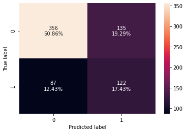
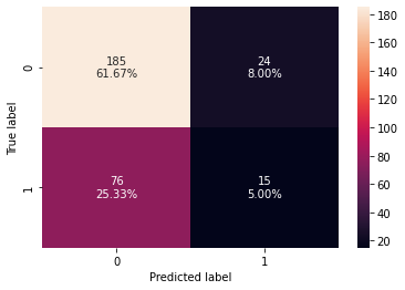
# creating confusion matrix
confusion_matrix_sklearn_with_threshold(lg, X_test, y_test)
In [53]:
log_reg_model_test_perf = model_performance_classification_sklearn_with_threshold(
    lg, X_test, y_test
)

print("Test set performance:")
log_reg_model_test_perf
Test set performance:
Out[53]:
| Accuracy | Recall | Precision | F1 | |
|---|---|---|---|---|
| 0 | 0.666667 | 0.164835 | 0.384615 | 0.230769 |
- ROC-AUC on test set
In [54]:
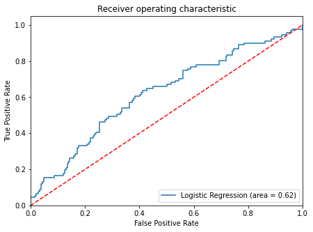
logit_roc_auc_test = roc_auc_score(y_test, lg.predict_proba(X_test)[:, 1])
fpr, tpr, thresholds = roc_curve(y_test, lg.predict_proba(X_test)[:, 1])
plt.figure(figsize=(7, 5))
plt.plot(fpr, tpr, label="Logistic Regression (area = %0.2f)" % logit_roc_auc_test)
plt.plot([0, 1], [0, 1], "r--")
plt.xlim([0.0, 1.0])
plt.ylim([0.0, 1.05])
plt.xlabel("False Positive Rate")
plt.ylabel("True Positive Rate")
plt.title("Receiver operating characteristic")
plt.legend(loc="lower right")
plt.show()
Using the model with threshold of 0.32
In [55]:
# creating confusion matrix
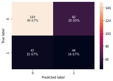
confusion_matrix_sklearn_with_threshold(
lg, X_test, y_test, threshold=optimal_threshold_auc_roc
)
In [56]:
# checking model performance for this model
log_reg_model_test_perf_threshold_auc_roc = model_performance_classification_sklearn_with_threshold(
    lg, X_test, y_test, threshold=optimal_threshold_auc_roc
)
print("Test set performance:")
log_reg_model_test_perf_threshold_auc_roc
Test set performance:
Out[56]:
| Accuracy | Recall | Precision | F1 | |
|---|---|---|---|---|
| 0 | 0.643333 | 0.483516 | 0.423077 | 0.451282 |
Using the model with threshold 0.34
In [57]:
# creating confusion matrix
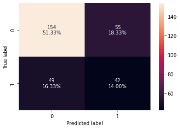
confusion_matrix_sklearn_with_threshold(
lg, X_test, y_test, threshold=optimal_threshold_curve
)
In [58]:
log_reg_model_test_perf_threshold_curve = model_performance_classification_sklearn_with_threshold(
    lg, X_test, y_test, threshold=optimal_threshold_curve
)
print("Test performance:")
log_reg_model_test_perf_threshold_curve
Test performance:
Out[58]:
| Accuracy | Recall | Precision | F1 | |
|---|---|---|---|---|
| 0 | 0.653333 | 0.461538 | 0.43299 | 0.446809 |
Model performance comparison
In [59]:
# training performance comparison

models_train_comp_df = pd.concat(
    [
        log_reg_model_train_perf.T,
        log_reg_model_train_perf_threshold_auc_roc.T,
        log_reg_model_train_perf_threshold_curve.T,
    ],
    axis=1,
)
models_train_comp_df.columns = [
    "Logistic Regression sklearn",
    "Logistic Regression-0.32 Threshold",
    "Logistic Regression-0.34 Threshold",
]

print("Training performance comparison:")
models_train_comp_df
Training performance comparison:
Out[59]:
| Logistic Regression sklearn | Logistic Regression-0.32 Threshold | Logistic Regression-0.34 Threshold | |
|---|---|---|---|
| Accuracy | 0.731429 | 0.682857 | 0.690000 |
| Recall | 0.244019 | 0.583732 | 0.550239 |
| Precision | 0.629630 | 0.474708 | 0.483193 |
| F1 | 0.351724 | 0.523605 | 0.514541 |
In [60]:
# testing performance comparison

models_test_comp_df = pd.concat(
    [
        log_reg_model_test_perf.T,
        log_reg_model_test_perf_threshold_auc_roc.T,
        log_reg_model_test_perf_threshold_curve.T,
    ],
    axis=1,
)
models_test_comp_df.columns = [
    "Logistic Regression sklearn",
    "Logistic Regression-0.32 Threshold",
    "Logistic Regression-0.34 Threshold",
]

print("Test set performance comparison:")
models_test_comp_df
Test set performance comparison:
Out[60]:
| Logistic Regression sklearn | Logistic Regression-0.32 Threshold | Logistic Regression-0.34 Threshold | |
|---|---|---|---|
| Accuracy | 0.666667 | 0.643333 | 0.653333 |
| Recall | 0.164835 | 0.483516 | 0.461538 |
| Precision | 0.384615 | 0.423077 | 0.432990 |
| F1 | 0.230769 | 0.451282 | 0.446809 |
Conclusion
- By changing the threshold of the logistic regression model we were able to see a significant improvement in the model performance.
- The model achieved a recall of 0.58 on the training set with threshold set at 0.32.
Recommendations
- From our logistic regression model we identified that Duration is a significant predictor of a customer being a defaulter.
- Bank should target more male customers as they have lesser odds of defaulting.
- We saw in our analysis that customers with a little or moderate amount in saving or checking accounts are more likely to default. The bank can be more strict with its rules or interest rates to compensate for the risk.
- We saw that customers who have rented or free housing are more likely to default. The bank should keep more details about such customers like hometown addresses, etc. to be able to track them.
- Our analysis showed that younger customers are slightly more likely to default. The bank can alter its policies to deal with this.