Data Analysis using Over Sampling and Under Sampling
Loan Delinquent Analysis
Context
DRS bank is facing challenging times. Their NPAs (Non-Performing Assets) have been on a rise recently and a large part of these are due to the loans given to individual customers(borrowers). The Chief Risk Officer of the bank decides to put in a scientifically robust framework for approval of loans to individual customers to minimize the risk of loans converting into NPAs and initiates a project for the data science team at the bank. You, as a senior member of the team, are assigned this project.
Objective
To identify the criteria to approve loans for an individual customer such that the likelihood of the loan delinquency is minimized
Key questions to be answered
What are the factors that drive the behavior of loan delinquency?
Data Description
- ID: Customer ID
- isDelinquent : indicates whether the customer is delinquent or not (1 => Yes, 0 => No)
- term: Loan term in months
- gender: Gender of the borrower
- age: Age of the borrower
- purpose: Purpose of Loan
- home_ownership: Status of borrower’s home
- FICO: FICO (i.e. the bureau score) of the borrower
Domain Information
Transactor – A person who pays his due amount balance full and on time.
Revolver – A person who pays the minimum due amount but keeps revolving his balance and does not pay the full amount.
Delinquent – Delinquency means that you are behind on payments, a person who fails to pay even the minimum due amount.
Defaulter – Once you are delinquent for a certain period your lender will declare you to be in the default stage.
Risk Analytics – A wide domain in the financial and banking industry, basically analyzing the risk of the customer.
Importing Libraries
In [1]:
# Libraries to help with reading and manipulating data
import numpy as np
import pandas as pd

# Libraries to help with data visualization
import matplotlib.pyplot as plt
import seaborn as sns

# To tune model, get different metric scores and split data
from sklearn.model_selection import GridSearchCV
from sklearn.model_selection import train_test_split, StratifiedKFold, cross_val_score
from sklearn.metrics import (
    f1_score,
    accuracy_score,
    recall_score,
    precision_score,
    confusion_matrix,
    roc_auc_score,
    plot_confusion_matrix,
)

# To build a logistic regression model
from sklearn.linear_model import LogisticRegression

# To use statistical functions
import scipy.stats as stats

# To oversample and undersample data
from imblearn.over_sampling import SMOTE
from imblearn.under_sampling import RandomUnderSampler

# To suppress the warning
import warnings

warnings.filterwarnings("ignore")

# This will help in making the Python code more structured automatically (good coding practice)
%load_ext nb_black
Loading Data
In [2]:
data = pd.read_csv("Loan_Delinquent_Dataset.csv")
In [3]:
# Checking the number of rows and columns in the data
data.shape
Out[3]:
(11548, 8)
Data Overview
In [4]:
# let's create a copy of the data
loan = data.copy()
In [5]:
# let's view the first 5 rows of the data
loan.head()
Out[5]:
| ID | isDelinquent | term | gender | purpose | home_ownership | age | FICO | |
|---|---|---|---|---|---|---|---|---|
| 0 | 1 | 1 | 36 months | Female | House | Mortgage | >25 | 300-500 |
| 1 | 2 | 0 | 36 months | Female | House | Rent | 20-25 | >500 |
| 2 | 3 | 1 | 36 months | Female | House | Rent | >25 | 300-500 |
| 3 | 4 | 1 | 36 months | Female | Car | Mortgage | >25 | 300-500 |
| 4 | 5 | 1 | 36 months | Female | House | Rent | >25 | 300-500 |
In [6]:
# let's view the last 5 rows of the data
loan.tail()
Out[6]:
| ID | isDelinquent | term | gender | purpose | home_ownership | age | FICO | |
|---|---|---|---|---|---|---|---|---|
| 11543 | 11544 | 0 | 60 months | Male | other | Mortgage | >25 | 300-500 |
| 11544 | 11545 | 1 | 36 months | Male | House | Rent | 20-25 | 300-500 |
| 11545 | 11546 | 0 | 36 months | Female | Personal | Mortgage | 20-25 | >500 |
| 11546 | 11547 | 1 | 36 months | Female | House | Rent | 20-25 | 300-500 |
| 11547 | 11548 | 1 | 36 months | Male | Personal | Mortgage | 20-25 | 300-500 |
In [7]:
# let's check the data types of the columns in the dataset
loan.info()
<class 'pandas.core.frame.DataFrame'>
RangeIndex: 11548 entries, 0 to 11547
Data columns (total 8 columns):
 #   Column          Non-Null Count  Dtype
---  ------          --------------  -----
 0   ID              11548 non-null  int64
 1   isDelinquent    11548 non-null  int64
 2   term            11548 non-null  object
 3   gender          11548 non-null  object
 4   purpose         11548 non-null  object
 5   home_ownership  11548 non-null  object
 6   age             11548 non-null  object
 7   FICO            11548 non-null  object
dtypes: int64(2), object(6)
memory usage: 721.9+ KB
Fixing the data types
- The term, gender, purpose,home_ownership, age and FICO are of object type, we can change them to categories.
converting "objects" to "category" reduces the data space required to store the dataframe
In [8]:
loan["term"] = loan["term"].astype("category")
loan["gender"] = loan["gender"].astype("category")
loan["purpose"] = loan["purpose"].astype("category")
loan["home_ownership"] = loan["home_ownership"].astype("category")
loan["age"] = loan["age"].astype("category")
loan["FICO"] = loan["FICO"].astype("category")
loan["isDelinquent"] = loan["isDelinquent"].astype("category")
In [9]:
loan.info()
<class 'pandas.core.frame.DataFrame'>
RangeIndex: 11548 entries, 0 to 11547
Data columns (total 8 columns):
 #   Column          Non-Null Count  Dtype
---  ------          --------------  -----
 0   ID              11548 non-null  int64
 1   isDelinquent    11548 non-null  category
 2   term            11548 non-null  category
 3   gender          11548 non-null  category
 4   purpose         11548 non-null  category
 5   home_ownership  11548 non-null  category
 6   age             11548 non-null  category
 7   FICO            11548 non-null  category
dtypes: category(7), int64(1)
memory usage: 170.2 KB
we can see that the memory usage has decreased from 721.9KB to 249.1KB
Observations
- All the dependent variables except for ID are categorical.
In [10]:
# let's check for duplicate values in the data
loan.duplicated().sum()
Out[10]:
0
In [11]:
# let's check for missing values in the data
loan.isnull().sum()
Out[11]:
ID                0
isDelinquent      0
term              0
gender            0
purpose           0
home_ownership    0
age               0
FICO              0
dtype: int64
- There are no missing values in the data
In [12]:
# let's view the statistical summary of the numerical columns in the data
loan.describe(include="all")
Out[12]:
| ID | isDelinquent | term | gender | purpose | home_ownership | age | FICO | |
|---|---|---|---|---|---|---|---|---|
| count | 11548.000000 | 11548.0 | 11548 | 11548 | 11548 | 11548 | 11548 | 11548 |
| unique | NaN | 2.0 | 2 | 2 | 7 | 3 | 2 | 2 |
| top | NaN | 1.0 | 36 months | Male | House | Mortgage | 20-25 | 300-500 |
| freq | NaN | 7721.0 | 10589 | 6555 | 6892 | 5461 | 5888 | 6370 |
| mean | 5774.500000 | NaN | NaN | NaN | NaN | NaN | NaN | NaN |
| std | 3333.764789 | NaN | NaN | NaN | NaN | NaN | NaN | NaN |
| min | 1.000000 | NaN | NaN | NaN | NaN | NaN | NaN | NaN |
| 25% | 2887.750000 | NaN | NaN | NaN | NaN | NaN | NaN | NaN |
| 50% | 5774.500000 | NaN | NaN | NaN | NaN | NaN | NaN | NaN |
| 75% | 8661.250000 | NaN | NaN | NaN | NaN | NaN | NaN | NaN |
| max | 11548.000000 | NaN | NaN | NaN | NaN | NaN | NaN | NaN |
Observations
- Most of the customers are loan delinquent(1)
- Most of the loans are for a 36-month term loan
- More males have applied for loans than females
- Most loan applications are for house loans
- Most customers have either mortgaged their houses
- Mostly customers in the age group 20-25 have applied for a loan
- Most customers have a FICO score between 300 and 500
Data Pre-Processing
In [13]:
# checking for unique values in the ID column
loan["ID"].nunique()
Out[13]:
11548
- Since all the values in the ID column are unique we can drop it
In [14]:
loan.drop(["ID"], axis=1, inplace=True)
In [15]:
# checking unique value in purpose
loan["purpose"].unique()
Out[15]:
['House', 'Car', 'Other', 'Personal', 'Wedding', 'Medical', 'other']
Categories (7, object): ['House', 'Car', 'Other', 'Personal', 'Wedding', 'Medical', 'other']
In [16]:
# We can merge the purpose -  'other' and 'Other' together
loan["purpose"].replace("other", "Other", inplace=True)
In [17]:
loan["purpose"].unique()
Out[17]:
['House', 'Car', 'Other', 'Personal', 'Wedding', 'Medical']
Categories (6, object): ['House', 'Car', 'Other', 'Personal', 'Wedding', 'Medical']
EDA
Univariate analysis
In [18]:
# function to create labeled barplots


def labeled_barplot(data, feature, perc=False, n=None):
    """
    Barplot with percentage at the top

    data: dataframe
    feature: dataframe column
    perc: whether to display percentages instead of count (default is False)
    n: displays the top n category levels (default is None, i.e., display all levels)
    """

    total = len(data[feature])  # length of the column
    count = data[feature].nunique()
    if n is None:
        plt.figure(figsize=(count + 1, 5))
    else:
        plt.figure(figsize=(n + 1, 5))

    plt.xticks(rotation=90, fontsize=15)
    ax = sns.countplot(
        data=data,
        x=feature,
        palette="Paired",
        order=data[feature].value_counts().index[:n].sort_values(),
    )

    for p in ax.patches:
        if perc == True:
            label = "{:.1f}%".format(
                100 * p.get_height() / total
            )  # percentage of each class of the category
        else:
            label = p.get_height()  # count of each level of the category

        x = p.get_x() + p.get_width() / 2  # width of the plot
        y = p.get_height()  # height of the plot

        ax.annotate(
            label,
            (x, y),
            ha="center",
            va="center",
            size=12,
            xytext=(0, 5),
            textcoords="offset points",
        )  # annotate the percentage

    plt.show()  # show the plot
Observations on isDelinquent
In [19]:
labeled_barplot(loan, "isDelinquent")
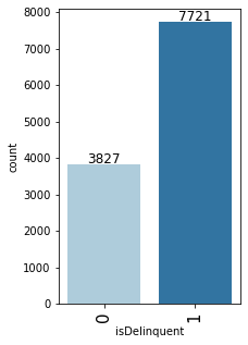
- 66% of the customers are delinquent
Observations on term
In [20]:
labeled_barplot(loan, "term")
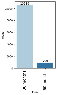
- 91.7% of the loans are for a 36-month term.
Observations on gender
In [21]:
labeled_barplot(loan, "gender")
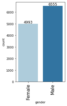
- There are more male applicants (56.8%) than female applicants (43.2%)
Observations on purpose
In [22]:
labeled_barplot(loan, "purpose")
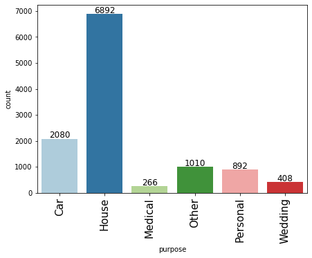
- Most loan applications are for house loans (59.7%) followed by car loans (18%)
- There are 2 levels named ‘other’ and ‘Other’ under the purpose variable. Since we do not have any other information about these, we can merge these levels.
Observations on home_ownership
In [23]:
labeled_barplot(loan, "home_ownership")
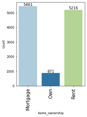
- Very few applicants <10% own their house, Most customers have either mortgaged their houses or live on rent.
Observations on age
In [24]:
labeled_barplot(loan, "age")
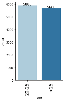
- Almost an equal percentage of people aged 20-25 and >25 have applied for the loan.
Observations on FICO
In [25]:
labeled_barplot(loan, "FICO")
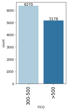
- Most customers have a FICO score between 300 and 500 (55.2%) followed by a score of greater than 500 (44.8%)
In [26]:
# function to plot stacked bar chart


def stacked_barplot(data, predictor, target):
    """
    Print the category counts and plot a stacked bar chart

    data: dataframe
    predictor: independent variable
    target: target variable
    """
    count = data[predictor].nunique()
    sorter = data[target].value_counts().index[-1]
    tab1 = pd.crosstab(data[predictor], data[target], margins=True).sort_values(
        by=sorter, ascending=False
    )
    print(tab1)
    print("-" * 120)
    tab = pd.crosstab(data[predictor], data[target], normalize="index").sort_values(
        by=sorter, ascending=False
    )
    tab.plot(kind="bar", stacked=True, figsize=(count + 1, 5))
    plt.legend(
        loc="lower left",
        frameon=False,
    )
    plt.legend(loc="upper left", bbox_to_anchor=(1, 1))
    plt.show()
In [27]:
stacked_barplot(loan, "term", "isDelinquent")
isDelinquent     0     1    All
term
All           3827  7721  11548
36 months     3168  7421  10589
60 months      659   300    959
------------------------------------------------------------------------------------------------------------------------
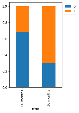
- Most loan delinquent customers have taken loans for 36 months.
In [28]:
stacked_barplot(loan, "gender", "isDelinquent")
isDelinquent     0     1    All
gender
All           3827  7721  11548
Male          1977  4578   6555
Female        1850  3143   4993
------------------------------------------------------------------------------------------------------------------------
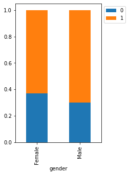
- There’s not much difference between male and female customers.
In [29]:
stacked_barplot(loan, "purpose", "isDelinquent")
isDelinquent     0     1    All
purpose
All           3827  7721  11548
House         2272  4620   6892
Car            678  1402   2080
Other          357   653   1010
Personal       274   618    892
Wedding        139   269    408
Medical        107   159    266
------------------------------------------------------------------------------------------------------------------------
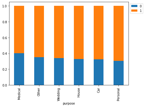
- Most loan delinquent customers are those who have applied for house loans followed by car and personal loans.
In [30]:
stacked_barplot(loan, "home_ownership", "isDelinquent")
isDelinquent       0     1    All
home_ownership
All             3827  7721  11548
Mortgage        1831  3630   5461
Rent            1737  3479   5216
Own              259   612    871
------------------------------------------------------------------------------------------------------------------------
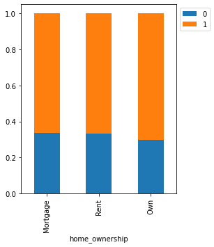
- Those customers who have their own house are less delinquent than the ones who live in a rented place or have mortgaged their home.
In [31]:
stacked_barplot(loan, "age", "isDelinquent")
isDelinquent     0     1    All
age
All           3827  7721  11548
>25           1969  3691   5660
20-25         1858  4030   5888
------------------------------------------------------------------------------------------------------------------------
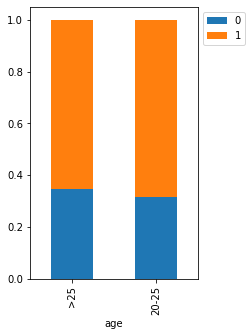
- Customers between 20-25 years of age are more delinquent.
In [32]:
stacked_barplot(loan, "FICO", "isDelinquent")
isDelinquent     0     1    All
FICO
All           3827  7721  11548
>500          2886  2292   5178
300-500        941  5429   6370
------------------------------------------------------------------------------------------------------------------------
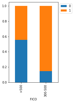
- If the FICO score is >500 the chances of delinquency decrease quite a lot compared to when the FICO score is between 300-500.
Key Observations
- FICO score and term of loan application appear to be very strong indicators of delinquency.
- Other factors appear to be not very good indicators of delinquency. (We can use chi-square tests to determine statistical significance in the association between two categorical variables).
We observed that a high FICO score means that the chances of delinquency are lower, let us see if any of the other variables indicate higher a FICO score.
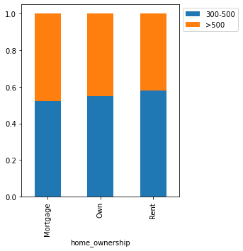
In [33]:
stacked_barplot(loan, "home_ownership", "FICO")
FICO            300-500  >500    All
home_ownership
All                6370  5178  11548
Mortgage           2857  2604   5461
Rent               3033  2183   5216
Own                 480   391    871
------------------------------------------------------------------------------------------------------------------------
In [34]:
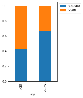
stacked_barplot(loan, "age", "FICO")
FICO   300-500  >500    All
age
All       6370  5178  11548
>25       2443  3217   5660
20-25     3927  1961   5888
------------------------------------------------------------------------------------------------------------------------
In [35]:
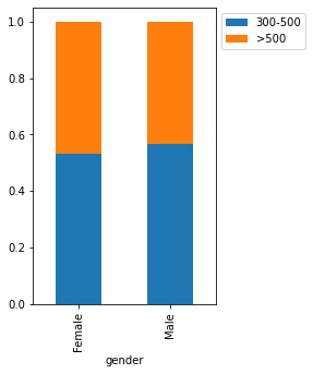
stacked_barplot(loan, "gender", "FICO")
FICO    300-500  >500    All
gender
All        6370  5178  11548
Male       3705  2850   6555
Female     2665  2328   4993
------------------------------------------------------------------------------------------------------------------------
Key Observations
- Home_ownership and gender seem to have a slight impact on the FICO scores.
- Age seems to have a much bigger impact on FICO scores.
Data Preparation for Modeling
In [39]:
x = loan.drop(["isDelinquent"], axis=1)
y = loan["isDelinquent"]
In [40]:
# encoding the categorical variables
x = pd.get_dummies(x, drop_first=True)
x.head()
Out[40]:
| term_60 months | gender_Male | purpose_House | purpose_Medical | purpose_Other | purpose_Personal | purpose_Wedding | home_ownership_Own | home_ownership_Rent | age_>25 | FICO_>500 | |
|---|---|---|---|---|---|---|---|---|---|---|---|
| 0 | 0 | 0 | 1 | 0 | 0 | 0 | 0 | 0 | 0 | 1 | 0 |
| 1 | 0 | 0 | 1 | 0 | 0 | 0 | 0 | 0 | 1 | 0 | 1 |
| 2 | 0 | 0 | 1 | 0 | 0 | 0 | 0 | 0 | 1 | 1 | 0 |
| 3 | 0 | 0 | 0 | 0 | 0 | 0 | 0 | 0 | 0 | 1 | 0 |
| 4 | 0 | 0 | 1 | 0 | 0 | 0 | 0 | 0 | 1 | 1 | 0 |
In [41]:
# Splitting data into training, validation and test set:
# first we split data into 2 parts, say temporary and test

X_temp, X_test, y_temp, y_test = train_test_split(
    x, y, test_size=0.2, random_state=1, stratify=y
)

# then we split the temporary set into train and validation

X_train, X_val, y_train, y_val = train_test_split(
    X_temp, y_temp, test_size=0.25, random_state=1, stratify=y_temp
)
print(X_train.shape, X_val.shape, X_test.shape)
(6928, 11) (2310, 11) (2310, 11)
In [42]:
print("Number of rows in train data =", X_train.shape[0])
print("Number of rows in validation data =", X_val.shape[0])
print("Number of rows in test data =", X_test.shape[0])
Number of rows in train data = 6928
Number of rows in validation data = 2310
Number of rows in test data = 2310
Building the model
Model evaluation criterion:
What does a bank want?
- A bank wants to minimize the loss – it can face 2 types of losses here:
- Whenever a bank lends money to a customer, they don’t return that.
- A bank doesn’t lend money to a customer thinking a customer will default but in reality, the customer won’t – opportunity loss.
Which loss is greater ?
- Lending to a customer who wouldn’t be able to pay back.
Since we want to reduce loan delinquency we should use Recall as a metric of model evaluation instead of accuracy.
- Recall – It gives the ratio of True positives to Actual positives, so high Recall implies low false negatives, i.e. low chances of predicting loan-delinquent customers as a non-loan-delinquent customer.
In [43]:
# defining a function to compute different metrics to check performance of a classification model built using sklearn
def model_performance_classification_sklearn(model, predictors, target):
    """
    Function to compute different metrics to check classification model performance

    model: classifier
    predictors: independent variables
    target: dependent variable
    """

    # predicting using the independent variables
    pred = model.predict(predictors)

    acc = accuracy_score(target, pred)  # to compute Accuracy
    recall = recall_score(target, pred)  # to compute Recall
    precision = precision_score(target, pred)  # to compute Precision
    f1 = f1_score(target, pred)  # to compute F1-score

    # creating a dataframe of metrics
    df_perf = pd.DataFrame(
        {
            "Accuracy": acc,
            "Recall": recall,
            "Precision": precision,
            "F1": f1,
        },
        index=[0],
    )

    return df_perf
In [44]:
def confusion_matrix_sklearn(model, predictors, target):
    """
    To plot the confusion_matrix with percentages

    model: classifier
    predictors: independent variables
    target: dependent variable
    """
    y_pred = model.predict(predictors)
    cm = confusion_matrix(target, y_pred)
    labels = np.asarray(
        [
            ["{0:0.0f}".format(item) + "\n{0:.2%}".format(item / cm.flatten().sum())]
            for item in cm.flatten()
        ]
    ).reshape(2, 2)

    plt.figure(figsize=(6, 4))
    sns.heatmap(cm, annot=labels, fmt="")
    plt.ylabel("True label")
    plt.xlabel("Predicted label")
Logistic Regression
In [45]:
lr = LogisticRegression(random_state=1)
lr.fit(X_train, y_train)
Out[45]:
LogisticRegression(random_state=1)
Let’s evaluate the model performance by using KFold and cross_val_score
K-Folds cross-validationprovides dataset indices to split data into train/validation sets. Split dataset into k consecutive stratified folds (without shuffling by default). Each fold is then used once as validation while the k – 1 remaining folds form the training set.
In [46]:
scoring = "recall"
kfold = StratifiedKFold(
    n_splits=5, shuffle=True, random_state=1
)  # Setting number of splits equal to 5
cv_result_bfr = cross_val_score(
    estimator=lr, X=X_train, y=y_train, scoring=scoring, cv=kfold
)
# Plotting boxplots for CV scores of model defined above
plt.boxplot(cv_result_bfr)
plt.show()
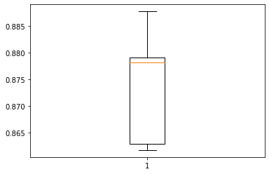
- Performance on training set varies between 0.86 to 0.87 recall.
- Let’s check the performance on validation data.
In [47]:
# Calculating different metrics on train set
log_reg_model_train_perf = model_performance_classification_sklearn(
    lr, X_train, y_train
)
print("Training performance:")
log_reg_model_train_perf
Training performance:
Out[47]:
| Accuracy | Recall | Precision | F1 | |
|---|---|---|---|---|
| 0 | 0.782621 | 0.872409 | 0.815375 | 0.842929 |
In [48]:
# Calculating different metrics on validation set
log_reg_model_val_perf = model_performance_classification_sklearn(lr, X_val, y_val)
print("Validation performance:")
log_reg_model_val_perf
Validation performance:
Out[48]:
| Accuracy | Recall | Precision | F1 | |
|---|---|---|---|---|
| 0 | 0.797403 | 0.891909 | 0.820727 | 0.854839 |
In [49]:
# creating confusion matrix
confusion_matrix_sklearn(lr, X_val, y_val)

- Logistic Regression has given a generalized performance on training and validation set.
- Let’s try oversampling (increase training data) to see if the model performance can be improved.
Oversampling train data using SMOTE
In [50]:
print("Before UpSampling, counts of label 'Yes': {}".format(sum(y_train == 1)))
print("Before UpSampling, counts of label 'No': {} \n".format(sum(y_train == 0)))

sm = SMOTE(
    sampling_strategy=1, k_neighbors=5, random_state=1
)  # Synthetic Minority Over Sampling Technique
X_train_over, y_train_over = sm.fit_resample(X_train, y_train)


print("After UpSampling, counts of label 'Yes': {}".format(sum(y_train_over == 1)))
print("After UpSampling, counts of label 'No': {} \n".format(sum(y_train_over == 0)))


print("After UpSampling, the shape of train_X: {}".format(X_train_over.shape))
print("After UpSampling, the shape of train_y: {} \n".format(y_train_over.shape))
Before UpSampling, counts of label 'Yes': 4632
Before UpSampling, counts of label 'No': 2296

After UpSampling, counts of label 'Yes': 4632
After UpSampling, counts of label 'No': 4632

After UpSampling, the shape of train_X: (9264, 11)
After UpSampling, the shape of train_y: (9264,)
Logistic Regression on oversampled data
In [51]:
log_reg_over = LogisticRegression(random_state=1)

# Training the basic logistic regression model with training set
log_reg_over.fit(X_train_over, y_train_over)
Out[51]:
LogisticRegression(random_state=1)
Let’s evaluate the model performance by using KFold and cross_val_score
K-Folds cross-validationprovides dataset indices to split data into train/validation sets. Split dataset into k consecutive stratified folds (without shuffling by default). Each fold is then used once as validation while the k – 1 remaining folds form the training set.
In [52]:
scoring = "recall"
kfold = StratifiedKFold(
    n_splits=5, shuffle=True, random_state=1
)  # Setting number of splits equal to 5
cv_result_over = cross_val_score(
    estimator=log_reg_over, X=X_train_over, y=y_train_over, scoring=scoring, cv=kfold
)
# Plotting boxplots for CV scores of model defined above
plt.boxplot(cv_result_over)
plt.show()
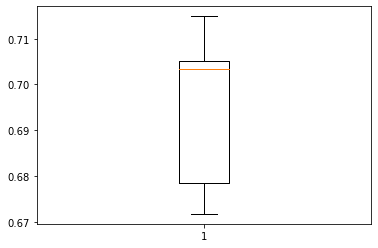
- Performance on training set varies between 0.69 to 0.70 recall
- Let’s check the performance on Validation set
In [53]:
# Calculating different metrics on train set
log_reg_over_train_perf = model_performance_classification_sklearn(
    log_reg_over, X_train_over, y_train_over
)
print("Training performance:")
log_reg_over_train_perf
Training performance:
Out[53]:
| Accuracy | Recall | Precision | F1 | |
|---|---|---|---|---|
| 0 | 0.769754 | 0.694732 | 0.817374 | 0.751079 |
In [54]:
# Calculating different metrics on validation set
log_reg_over_val_perf = model_performance_classification_sklearn(
    log_reg_over, X_val, y_val
)
print("validation performance:")
log_reg_over_val_perf
validation performance:
Out[54]:
| Accuracy | Recall | Precision | F1 | |
|---|---|---|---|---|
| 0 | 0.760606 | 0.719094 | 0.903252 | 0.800721 |
In [55]:
# creating confusion matrix
confusion_matrix_sklearn(log_reg_over, X_val, y_val)
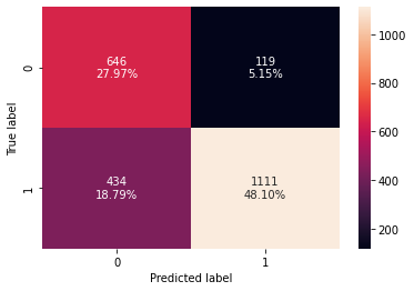
- Performance on the training set improved but the model is not able to replicate the same for the validation set.
- Model is overfitting.
- Lets try:a) Regularization to see if overfitting can be reducedb) Undersampling the train to handle the imbalance between classes and check the model performance.
Regularization
In [56]:
# Choose the type of classifier.
lr_estimator = LogisticRegression(random_state=1, solver="saga")

# Grid of parameters to choose from
parameters = {"C": np.arange(0.1, 1.1, 0.1)}

# Run the grid search
grid_obj = GridSearchCV(lr_estimator, parameters, scoring="recall")
grid_obj = grid_obj.fit(X_train_over, y_train_over)

# Set the clf to the best combination of parameters
lr_estimator = grid_obj.best_estimator_

# Fit the best algorithm to the data.
lr_estimator.fit(X_train_over, y_train_over)
Out[56]:
LogisticRegression(C=0.1, random_state=1, solver='saga')
In [57]:
# Calculating different metrics on train set
log_reg_reg_train_perf = model_performance_classification_sklearn(
    lr_estimator, X_train_over, y_train_over
)
print("Training performance:")
log_reg_reg_train_perf
Training performance:
Out[57]:
| Accuracy | Recall | Precision | F1 | |
|---|---|---|---|---|
| 0 | 0.739313 | 0.694732 | 0.76274 | 0.727149 |
In [58]:
# Calculating different metrics on validation set
log_reg_reg_val_perf = model_performance_classification_sklearn(
    lr_estimator, X_val, y_val
)
print("Validation performance:")
log_reg_reg_val_perf
Validation performance:
Out[58]:
| Accuracy | Recall | Precision | F1 | |
|---|---|---|---|---|
| 0 | 0.748918 | 0.719094 | 0.88385 | 0.793005 |
In [59]:
# creating confusion matrix
confusion_matrix_sklearn(lr_estimator, X_val, y_val)
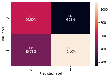
- Recall is very good, but similar to previous model
Undersampling train data using RandomUnderSampler
In [60]:
rus = RandomUnderSampler(random_state=1)
X_train_un, y_train_un = rus.fit_resample(X_train, y_train)
In [61]:
print("Before Under Sampling, counts of label 'Yes': {}".format(sum(y_train == 1)))
print("Before Under Sampling, counts of label 'No': {} \n".format(sum(y_train == 0)))

print("After Under Sampling, counts of label 'Yes': {}".format(sum(y_train_un == 1)))
print("After Under Sampling, counts of label 'No': {} \n".format(sum(y_train_un == 0)))

print("After Under Sampling, the shape of train_X: {}".format(X_train_un.shape))
print("After Under Sampling, the shape of train_y: {} \n".format(y_train_un.shape))
Before Under Sampling, counts of label 'Yes': 4632
Before Under Sampling, counts of label 'No': 2296

After Under Sampling, counts of label 'Yes': 2296
After Under Sampling, counts of label 'No': 2296

After Under Sampling, the shape of train_X: (4592, 11)
After Under Sampling, the shape of train_y: (4592,)
Logistic Regression on undersampled data
In [62]:
log_reg_under = LogisticRegression(random_state=1)
log_reg_under.fit(X_train_un, y_train_un)
Out[62]:
LogisticRegression(random_state=1)
Let’s evaluate the model performance by using KFold and cross_val_score
K-Folds cross-validationprovides dataset indices to split data into train/validation sets. Split dataset into k consecutive stratified folds (without shuffling by default). Each fold is then used once as validation while the k – 1 remaining folds form the training set.
In [63]:
scoring = "recall"
kfold = StratifiedKFold(
    n_splits=5, shuffle=True, random_state=1
)  # Setting number of splits equal to 5
cv_result_under = cross_val_score(
    estimator=log_reg_under, X=X_train_un, y=y_train_un, scoring=scoring, cv=kfold
)
# Plotting boxplots for CV scores of model defined above
plt.boxplot(cv_result_under)
plt.show()
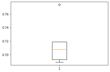
- Performance of model on training set varies between 0.70 to 0.76, which is similar to model with oversampled data
- Let’s check the performance on the validation set.
In [64]:
# Calculating different metrics on train set
log_reg_under_train_perf = model_performance_classification_sklearn(
    log_reg_under, X_train_un, y_train_un
)
print("Training performance:")
log_reg_under_train_perf
Training performance:
Out[64]:
| Accuracy | Recall | Precision | F1 | |
|---|---|---|---|---|
| 0 | 0.768075 | 0.708624 | 0.804251 | 0.753415 |
In [65]:
# Calculating different metrics on validation set
log_reg_under_val_perf = model_performance_classification_sklearn(
    log_reg_under, X_val, y_val
)
print("Validation performance:")
log_reg_under_val_perf
Validation performance:
Out[65]:
| Accuracy | Recall | Precision | F1 | |
|---|---|---|---|---|
| 0 | 0.769264 | 0.739806 | 0.897174 | 0.810926 |
In [66]:
# creating confusion matrix
confusion_matrix_sklearn(log_reg_under, X_val, y_val)
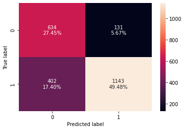
- Model has given a generalized performance on training and validation set.
- Model performance has improved using downsampling – Logistic regression is now able to differentiate well between positive and negative classes.
In [67]:
# training performance comparison

models_train_comp_df = pd.concat(
    [
        log_reg_model_train_perf.T,
        log_reg_over_train_perf.T,
        log_reg_reg_train_perf.T,
        log_reg_under_train_perf.T,
    ],
    axis=1,
)
models_train_comp_df.columns = [
    "Logistic Regression",
    "Logistic Regression with oversampled data",
    "Regularised Logistic Regression",
    "Logistic Regression with undersampled data",
]
print("Training performance comparison:")
models_train_comp_df
Training performance comparison:
Out[67]:
| Logistic Regression | Logistic Regression with oversampled data | Regularised Logistic Regression | Logistic Regression with undersampled data | |
|---|---|---|---|---|
| Accuracy | 0.782621 | 0.769754 | 0.739313 | 0.768075 |
| Recall | 0.872409 | 0.694732 | 0.694732 | 0.708624 |
| Precision | 0.815375 | 0.817374 | 0.762740 | 0.804251 |
| F1 | 0.842929 | 0.751079 | 0.727149 | 0.753415 |
In [68]:
# Validation performance comparison

models_train_comp_df = pd.concat(
    [
        log_reg_model_val_perf.T,
        log_reg_over_val_perf.T,
        log_reg_reg_val_perf.T,
        log_reg_under_val_perf.T,
    ],
    axis=1,
)
models_train_comp_df.columns = [
    "Logistic Regression",
    "Logistic Regression with oversampled data",
    "Regularised Logistic Regression",
    "Logistic Regression with undersampled data",
]
print("Validation performance comparison:")
models_train_comp_df
Validation performance comparison:
Out[68]:
| Logistic Regression | Logistic Regression with oversampled data | Regularised Logistic Regression | Logistic Regression with undersampled data | |
|---|---|---|---|---|
| Accuracy | 0.797403 | 0.760606 | 0.748918 | 0.769264 |
| Recall | 0.891909 | 0.719094 | 0.719094 | 0.739806 |
| Precision | 0.820727 | 0.903252 | 0.883850 | 0.897174 |
| F1 | 0.854839 | 0.800721 | 0.793005 | 0.810926 |
- Initial logistic regression without sampling and regularization has given a generalized performance on training and validation set.
We can see that first model is the best, let’s check the performance of test data
In [69]:
# Calculating different metrics on validation set
log_reg_model_test_perf = model_performance_classification_sklearn(
    log_reg_under, X_test, y_test
)
print("Test performance:")
log_reg_model_test_perf
Test performance:
Out[69]:
| Accuracy | Recall | Precision | F1 | |
|---|---|---|---|---|
| 0 | 0.765368 | 0.733808 | 0.896361 | 0.80698 |
In [70]:
# creating confusion matrix
confusion_matrix_sklearn(lr, X_test, y_test)
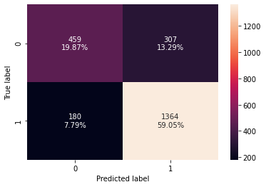
- Model has given generalised performance on the test set
Business Insights
- FICO, term and gender are the important variables in determining if a borrower will get into a delinquent stage
- No borrower shall be given a loan if they are applying for a 36-month term loan and have a FICO score in the range of 300-500.
- Female borrowers with a FICO score greater than 500 should be our target customers.