Data Analysis using Pandas in Python

Pandas is a very popular Python library to perform analysis of tabular data. In data science jargon, such tables are referred to as dataframes. Pandas provide various functionalities to create insightful business advices. Let’s start from the basics and slowly progress towards complex use cases.

1.1 Pandas – Series and DataFrames

Pandas Series

• Pandas Series is a one-dimensional labeled array/list capable of holding data of any type (integer, string, float, python objects, etc.). 
• The labels are collectively called index. 
• Pandas Series can be thought as a single column of an excel spreadsheet and each entry in a series corresponds to an individual row in the spreadsheet.

# creating a list of price of different medicines
med_price_list = [55,25,75,40,90]

# converting the med_price_list to an array 
med_price_arr = np.array(med_price_list)

# converting the list and array into a Pandas Series object  
series_list = pd.Series(med_price_list)
series_arr = pd.Series(med_price_arr)

# printing the converted series object
print(series_list)
print(series_arr)

Output

0    55
1    25
2    75
3    40
4    90
dtype: int64
0    55
1    25
2    75
3    40
4    90
dtype: int64

• We can see that the list and array have been converted to a Pandas Series object.
• We also see that the series has automatically got index labels. Let’s see how these can be modified.

# changing the index of a series
med_price_list_labeled = pd.Series(med_price_list, index = ['Omeprazole','Azithromycin','Metformin','Ibuprofen','Cetirizine'])
print(med_price_list_labeled)

Output

Omeprazole      55
Azithromycin    25
Metformin       75
Ibuprofen       40
Cetirizine      90
dtype: int64

1.2 Performing mathematical operations on Pandas Series

The price of each medicine was increased by $2.5. Let’s add this to the existing price.

# adding 2.5 to existing prices
med_price_list_labeled_updated = med_price_list_labeled + 2.5
med_price_list_labeled_updated

Output

Omeprazole      57.5
Azithromycin    27.5
Metformin       77.5
Ibuprofen       42.5
Cetirizine      92.5
dtype: float64

• A new price list was released by vendors for each medicine. Let’s find the difference between new price and the old price

new_price_list = [77, 45.5, 100, 50, 80]
new_price_list_labeled = pd.Series(new_price_list, index = ['Omeprazole','Azithromycin','Metformin','Ibuprofen','Cetirizine'])
print(new_price_list_labeled)

Output

Omeprazole       77.0
Azithromycin     45.5
Metformin       100.0
Ibuprofen        50.0
Cetirizine       80.0
dtype: float64

print('Difference between new price and old price - ')
print(new_price_list_labeled - med_price_list_labeled_updated)

Difference between new price and old price - 
Omeprazole      19.5
Azithromycin    18.0
Metformin       22.5
Ibuprofen        7.5
Cetirizine     -12.5
dtype: float64

1.3 Creating a Pandas DataFrame using a list

student = ['Mary', 'Peter', 'Susan', 'Toby', 'Vishal']
df1 = pd.DataFrame(student,columns=['Student'])
df1

Out[66]:

	Student
0	Mary
1	Peter
2	Susan
3	Toby
4	Vishal

1.4 Creating a Pandas DataFrame using a dictionary

# defining another list
grades = ['B-','A+','A-', 'B+', 'C']

# creating the dataframe using a dictionary
df2 = pd.DataFrame({'Student':student,'Grade':grades})
df2

Output

	Student	Grade
0	Mary	B-
1	Peter	A+
2	Susan	A-
3	Toby	B+
4	Vishal	C

1.5 Creating a Pandas DataFrame using Series

The data for total energy consumption for the U.S. was collected from 2012 – 2018. Let’s see how this data can be presented in form of data frame.

year = pd.Series([2012,2013,2014,2015,2016,2017,2018])
energy_consumption = pd.Series([2152,2196,2217,2194,2172,2180,2258])

df3 = pd.DataFrame({'Year':year,'Energy_Consumption(Mtoe)':energy_consumption})
df3

Output

	Year	Energy_Consumption(Mtoe)
0	2012	2152
1	2013	2196
2	2014	2217
3	2015	2194
4	2016	2172
5	2017	2180
6	2018	2258

1.6 Creating a Pandas DataFrame using random values

For encryption purposes a web browser company wants to generate random values which have mean equal to 0 and variance equal to 1. They want 5 randomly generated numbers in 2 different trials.

# we can create a new dataframe using random values 
df4 = pd.DataFrame(np.random.randn(5,2),columns = ['Trial 1', 'Trial 2'])
df4

Output

	Trial 1	Trial 2
0	0.956411	0.292236
1	-0.292173	0.730664
2	0.107673	1.493363
3	-1.156195	0.269528
4	0.091713	0.153680

1.7 Pandas – Accessing and Modifying

Accessing Series

The revenue (in billion dollars) of different telecommunication operators in U.S. was collected for the year of 2020. The following lists consist of the names of the telecommunication operators and their respective revenue (in billion dollars).

operators = ['AT&T', 'Verizon', 'T-Mobile US', 'US Cellular']
revenue = [171.76, 128.29, 68.4, 4.04]

#creating a Series from lists
telecom = pd.Series(revenue, index=operators)
telecom

Output

AT&T           171.76
Verizon        128.29
T-Mobile US     68.40
US Cellular      4.04
dtype: float64

Accessing Pandas Series using its index

# accessing the first element of series 
telecom[0]

Output

171.76

#  accessing firt 3 elements of a series
telecom[:3]

Output

AT&T           171.76
Verizon        128.29
T-Mobile US     68.40
dtype: float64

# accessing the last two elements of a series
telecom[-2:]

Output

T-Mobile US    68.40
US Cellular     4.04
dtype: float64

# accessing multiple elements of a series
telecom[[0,2,3]]

Output

AT&T           171.76
T-Mobile US     68.40
US Cellular      4.04
dtype: float64

Accessing Pandas Series using its labeled index

# accessing the revenue of AT&T
telecom['AT&T']

Output

171.76

#  accessing firt 3 revenues of operators in the series
telecom[:'T-Mobile US']

Output

AT&T           171.76
Verizon        128.29
T-Mobile US     68.40
dtype: float64

# accessing multiple values
telecom[['AT&T','US Cellular','Verizon']]

Output

AT&T           171.76
US Cellular      4.04
Verizon        128.29
dtype: float64

Accessing DataFrames

The data of the customers visiting 24/7 Stores from different locations was collected. The data includes Customer ID, location of store, gender of the customer, type of product purchased, quantity of products purchased, total bill amount. Let’s create the dataset and see how to access different entries of it.

# creating the dataframe using dictionary
store_data = pd.DataFrame({'CustomerID': ['CustID00','CustID01','CustID02','CustID03','CustID04']
                           ,'location': ['Chicago', 'Boston', 'Seattle', 'San Francisco', 'Austin']
                           ,'gender': ['M','M','F','M','F']
                           ,'type': ['Electronics','Food&Beverages','Food&Beverages','Medicine','Beauty']
                           ,'quantity':[1,3,4,2,1],'total_bill':[100,75,125,50,80]})
store_data

Output

	CustomerID	location	gender	type	quantity	total_bill
0	CustID00	Chicago	M	Electronics	1	100
1	CustID01	Boston	M	Food&Beverages	3	75
2	CustID02	Seattle	F	Food&Beverages	4	125
3	CustID03	San Francisco	M	Medicine	2	50
4	CustID04	Austin	F	Beauty	1	80

# accessing first row of the dataframe
store_data[:1]

Output

	CustomerID	location	gender	type	quantity	total_bill
0	CustID00	Chicago	M	Electronics	1	100

# accessing first column of the dataframe
store_data['location']

Output

0          Chicago
1           Boston
2          Seattle
3    San Francisco
4           Austin
Name: location, dtype: object

# accessing rows with the step size of 2
store_data[::2] 

Output

	CustomerID	location	gender	type	quantity	total_bill
0	CustID00	Chicago	M	Electronics	1	100
2	CustID02	Seattle	F	Food&Beverages	4	125
4	CustID04	Austin	F	Beauty	1	80

# accessing the rows in reverse
store_data[::-2]

Output

	CustomerID	location	gender	type	quantity	total_bill
4	CustID04	Austin	F	Beauty	1	80
2	CustID02	Seattle	F	Food&Beverages	4	125
0	CustID00	Chicago	M	Electronics	1	100

Using loc and iloc method

loc method

• loc is a method to access rows and columns on pandas objects. When using the loc method on a dataframe, we specify which rows and which columns we want by using the following format:
  • dataframe.loc[row selection, column selection]
• DataFrame.loc[] method is a method that takes only index labels and returns row or dataframe if the index label exists in the data frame.

# accessing first index value using loc method (indexing starts from 0 in python)
store_data.loc[1]

Output

CustomerID          CustID01
location              Boston
gender                     M
type          Food&Beverages
quantity                   3
total_bill                75
Name: 1, dtype: object

Accessing selected rows and columns using loc method

# accessing 1st and 4th index values along with location and type columns 
store_data.loc[[1,4],['location','type']]

Output

	location	type
1	Boston	Food&Beverages
4	Austin	Beauty

iloc method

• The iloc indexer for Pandas Dataframe is used for integer location-basedindexing/selection by position. When using the loc method on a dataframe, we specify which rows and which columns we want by using the following format:
  • dataframe.iloc[row selection, column selection]

# accessing selected rows and columns using iloc method 
store_data.iloc[[1,4],[0,2]]

Output

	CustomerID	gender
1	CustID01	M
4	CustID04	F

Difference between loc and iloc indexing methods

• loc is label-based, which means that you have to specify rows and columns based on their row and column labels.
• iloc is integer position-based, so you have to specify rows and columns by their integer position values (0-based integer position).

If we use labels instead of index values in .iloc it will throw an error.

# accessing selected rows and columns using iloc method 
store_data.iloc[[1,4],['location','type']]

---------------------------------------------------------------------------
IndexError                                Traceback (most recent call last)
<ipython-input-89-53acc0d7ec5b> in <module>()
      1 # accessing selected rows and columns using iloc method
----> 2 store_data.iloc[[1,4],['location','type']]

/usr/local/lib/python3.7/dist-packages/pandas/core/indexing.py in __getitem__(self, key)
    871                     # AttributeError for IntervalTree get_value
    872                     pass
--> 873             return self._getitem_tuple(key)
    874         else:
    875             # we by definition only have the 0th axis

/usr/local/lib/python3.7/dist-packages/pandas/core/indexing.py in _getitem_tuple(self, tup)
   1441     def _getitem_tuple(self, tup: Tuple):
   1442 
-> 1443         self._has_valid_tuple(tup)
   1444         try:
   1445             return self._getitem_lowerdim(tup)

/usr/local/lib/python3.7/dist-packages/pandas/core/indexing.py in _has_valid_tuple(self, key)
    700                 raise IndexingError("Too many indexers")
    701             try:
--> 702                 self._validate_key(k, i)
    703             except ValueError as err:
    704                 raise ValueError(

/usr/local/lib/python3.7/dist-packages/pandas/core/indexing.py in _validate_key(self, key, axis)
   1361             # check that the key has a numeric dtype
   1362             if not is_numeric_dtype(arr.dtype):
-> 1363                 raise IndexError(f".iloc requires numeric indexers, got {arr}")
   1364 
   1365             # check that the key does not exceed the maximum size of the index

IndexError: .iloc requires numeric indexers, got ['location' 'type']

• As expected, .iloc has given error on using ‘labels’.

We can modify entries of a dataframe using loc or iloc too

print(store_data.loc[4,'type'])
store_data.loc[4,'type'] = 'Electronics'

Electronics

store_data

Output

	CustomerID	location	gender	type	quantity	total_bill
0	CustID00	Chicago	M	Electronics	1	100
1	CustID01	Boston	M	Food&Beverages	3	75
2	CustID02	Seattle	F	Food&Beverages	4	125
3	CustID03	San Francisco	M	Medicine	2	50
4	CustID04	Austin	F	Electronics	1	80

store_data.iloc[4,3] = 'Beauty'
store_data

Output

	CustomerID	location	gender	type	quantity	total_bill
0	CustID00	Chicago	M	Electronics	1	100
1	CustID01	Boston	M	Food&Beverages	3	75
2	CustID02	Seattle	F	Food&Beverages	4	125
3	CustID03	San Francisco	M	Medicine	2	50
4	CustID04	Austin	F	Beauty	1	80

Condition based indexing

store_data['quantity']>1

Output

0    False
1     True
2     True
3     True
4    False
Name: quantity, dtype: bool

• Wherever the condition of greater than 1 is satisfied in quantity column, ‘True’ is returned. Let’s retrieve the original values wherever the condition is satisfied.

store_data.loc[store_data['quantity']>1]

Output

	CustomerID	location	gender	type	quantity	total_bill
1	CustID01	Boston	M	Food&Beverages	3	75
2	CustID02	Seattle	F	Food&Beverages	4	125
3	CustID03	San Francisco	M	Medicine	2	50

• Wherever the condition is satisfied we get the original values, and wherever the condition is not satisfied we do not get those records in the output.

Column addition and removal from a Pandas DataFrame

Adding a new column in a DataFrame

store_data

Output

	CustomerID	location	gender	type	quantity	total_bill
0	CustID00	Chicago	M	Electronics	1	100
1	CustID01	Boston	M	Food&Beverages	3	75
2	CustID02	Seattle	F	Food&Beverages	4	125
3	CustID03	San Francisco	M	Medicine	2	50
4	CustID04	Austin	F	Beauty	1	80

# adding a new column in data frame store_data which is a rating (out of 5) given by customer based on their shopping experience
store_data['rating'] = [2,5,3,4,4]
store_data

Output

	CustomerID	location	gender	type	quantity	total_bill	rating
0	CustID00	Chicago	M	Electronics	1	100	2
1	CustID01	Boston	M	Food&Beverages	3	75	5
2	CustID02	Seattle	F	Food&Beverages	4	125	3
3	CustID03	San Francisco	M	Medicine	2	50	4
4	CustID04	Austin	F	Beauty	1	80	4

Removing a column from a DataFrame

• The CustomerID column is a unique identifier of each customer. This unique identifier will not help 24/7 Stores in getting useful insights about their customers. So, they have decided to remove this column from the data frame.

store_data.drop('CustomerID',axis=1)

Output

	location	gender	type	quantity	total_bill	rating
0	Chicago	M	Electronics	1	100	2
1	Boston	M	Food&Beverages	3	75	5
2	Seattle	F	Food&Beverages	4	125	3
3	San Francisco	M	Medicine	2	50	4
4	Austin	F	Beauty	1	80	4

• We sucessfully removed the ‘CustomerID’ from dataframe. But this change is not permanent in the dataframe, let’s have a look at the store_data again.

store_data

Output

	CustomerID	location	gender	type	quantity	total_bill	rating
0	CustID00	Chicago	M	Electronics	1	100	2
1	CustID01	Boston	M	Food&Beverages	3	75	5
2	CustID02	Seattle	F	Food&Beverages	4	125	3
3	CustID03	San Francisco	M	Medicine	2	50	4
4	CustID04	Austin	F	Beauty	1	80	4

• We see that store_data still has column ‘CustomerID’ in it. 
• To make permanent changes to a dataframe there are two methods will have to use a parameter inplace and set its value to True.

store_data.drop('CustomerID',axis=1,inplace=True)
store_data

Output

	location	gender	type	quantity	total_bill	rating
0	Chicago	M	Electronics	1	100	2
1	Boston	M	Food&Beverages	3	75	5
2	Seattle	F	Food&Beverages	4	125	3
3	San Francisco	M	Medicine	2	50	4
4	Austin	F	Beauty	1	80	4

• Now the column has been permanently removed from the dataframe.

# we can also remove multiple columns simultaneously 
# it is always a good idea to store the new/updated data frames in new variables to avoid changes to the existing data frame

# creating a copy of the existing data frame
new_store_data = store_data.copy()
store_data

Output

	location	gender	type	quantity	total_bill	rating
0	Chicago	M	Electronics	1	100	2
1	Boston	M	Food&Beverages	3	75	5
2	Seattle	F	Food&Beverages	4	125	3
3	San Francisco	M	Medicine	2	50	4
4	Austin	F	Beauty	1	80	4

# dropping location and rating columns simultaneously
new_store_data.drop(['location','rating'],axis=1,inplace=True)
new_store_data

Output

	gender	type	quantity	total_bill
0	M	Electronics	1	100
1	M	Food&Beverages	3	75
2	F	Food&Beverages	4	125
3	M	Medicine	2	50
4	F	Beauty	1	80

# lets check if store_data was impacted
store_data

Output

	location	gender	type	quantity	total_bill	rating
0	Chicago	M	Electronics	1	100	2
1	Boston	M	Food&Beverages	3	75	5
2	Seattle	F	Food&Beverages	4	125	3
3	San Francisco	M	Medicine	2	50	4
4	Austin	F	Beauty	1	80	4

• There were no changes to data frame store_data.

• Deep copy stores copies of the object’s value.
• Shallow Copy stores the references of objects to the original memory address. 

Removing rows from a dataframe

store_data.drop(1,axis=0)

Output

	location	gender	type	quantity	total_bill	rating
0	Chicago	M	Electronics	1	100	2
2	Seattle	F	Food&Beverages	4	125	3
3	San Francisco	M	Medicine	2	50	4
4	Austin	F	Beauty	1	80	4

store_data

Output

	location	gender	type	quantity	total_bill	rating
0	Chicago	M	Electronics	1	100	2
1	Boston	M	Food&Beverages	3	75	5
2	Seattle	F	Food&Beverages	4	125	3
3	San Francisco	M	Medicine	2	50	4
4	Austin	F	Beauty	1	80	4

• Notice that we used axis=0 to drop a row from a data frame, while we were using axis=1 for dropping a column from the data frame.
• Also, to make permanent changes to the data frame we will have to use inplace=True parameter.
• We also see that the index are not correct now as first row has been removed. So, we will have to reset the index of the data frame. Let’s see how this can be done.

# creating a new dataframe
store_data_new  = store_data.drop(1,axis=0)
store_data_new

Output

	location	gender	type	quantity	total_bill	rating
0	Chicago	M	Electronics	1	100	2
2	Seattle	F	Food&Beverages	4	125	3
3	San Francisco	M	Medicine	2	50	4
4	Austin	F	Beauty	1	80	4

# resetting the index of data frame
store_data_new.reset_index()

Output

	index	location	gender	type	quantity	total_bill	rating
0	0	Chicago	M	Electronics	1	100	2
1	2	Seattle	F	Food&Beverages	4	125	3
2	3	San Francisco	M	Medicine	2	50	4
3	4	Austin	F	Beauty	1	80	4

• We see that the index of the data frame is now resetted but the index has become a column in the data frame. We do not need the index to become a column so we can simply set the parameter drop=True in reset_index() function.

# setting inplace = True to make the changes permanent
store_data_new.reset_index(drop=True,inplace=True)
store_data_new

Output

	location	gender	type	quantity	total_bill	rating
0	Chicago	M	Electronics	1	100	2
1	Seattle	F	Food&Beverages	4	125	3
2	San Francisco	M	Medicine	2	50	4
3	Austin	F	Beauty	1	80	4

1.8 Pandas – Combining DataFrames

We will examine 3 methods for combining dataframes

1. concat
2. join
3. merge

data_cust = pd.DataFrame({"customerID":['101','102','103','104'], 
                        'category': ['Medium','Medium','High','Low'],
                        'first_visit': ['yes','no','yes','yes'],
                        'sales': [123,52,214,663]},index=[0,1,2,3])

data_cust_new = pd.DataFrame({"customerID":['101','103','104','105'], 
                    'distance': [12,9,44,21],
                    'sales': [123,214,663,331]},index=[4,5,6,7])

data_cust

Output

	customerID	category	first_visit	sales
0	101	Medium	yes	123
1	102	Medium	no	52
2	103	High	yes	214
3	104	Low	yes	663

data_cust_new

Output

	customerID	distance	sales
4	101	12	123
5	103	9	214
6	104	44	663
7	105	21	331

pd.concat([data_cust,data_cust_new],axis=0)

Output

	customerID	category	first_visit	sales	distance
0	101	Medium	yes	123	NaN
1	102	Medium	no	52	NaN
2	103	High	yes	214	NaN
3	104	Low	yes	663	NaN
4	101	NaN	NaN	123	12.0
5	103	NaN	NaN	214	9.0
6	104	NaN	NaN	663	44.0
7	105	NaN	NaN	331	21.0

pd.concat([data_cust,data_cust_new],axis=1)

Output

	customerID	category	first_visit	sales	customerID	distance	sales
0	101	Medium	yes	123.0	NaN	NaN	NaN
1	102	Medium	no	52.0	NaN	NaN	NaN
2	103	High	yes	214.0	NaN	NaN	NaN
3	104	Low	yes	663.0	NaN	NaN	NaN
4	NaN	NaN	NaN	NaN	101	12.0	123.0
5	NaN	NaN	NaN	NaN	103	9.0	214.0
6	NaN	NaN	NaN	NaN	104	44.0	663.0
7	NaN	NaN	NaN	NaN	105	21.0	331.0

Merge and Join

• Merge combines dataframes using a column’s values to identify common entries
• Join combines dataframes using the index to identify common entries

pd.merge(data_cust,data_cust_new,how='outer',on='customerID') # outer merge is union of on

Output

	customerID	category	first_visit	sales_x	distance	sales_y
0	101	Medium	yes	123.0	12.0	123.0
1	102	Medium	no	52.0	NaN	NaN
2	103	High	yes	214.0	9.0	214.0
3	104	Low	yes	663.0	44.0	663.0
4	105	NaN	NaN	NaN	21.0	331.0

pd.merge(data_cust,data_cust_new,how='inner',on='customerID') # inner merge is intersection of on

Output

	customerID	category	first_visit	sales_x	distance	sales_y
0	101	Medium	yes	123	12	123
1	103	High	yes	214	9	214
2	104	Low	yes	663	44	663

pd.merge(data_cust,data_cust_new,how='right',on='customerID') 

Output

	customerID	category	first_visit	sales_x	distance	sales_y
0	101	Medium	yes	123.0	12	123
1	103	High	yes	214.0	9	214
2	104	Low	yes	663.0	44	663
3	105	NaN	NaN	NaN	21	331

data_quarters = pd.DataFrame({'Q1': [101,102,103],
                              'Q2': [201,202,203]},
                               index=['I0','I1','I2'])

data_quarters_new = pd.DataFrame({'Q3': [301,302,303],
                                  'Q4': [401,402,403]},
                               index=['I0','I2','I3'])

data_quarters

Output

	Q1	Q2
I0	101	201
I1	102	202
I2	103	203

data_quarters_new

Output

	Q3	Q4
I0	301	401
I2	302	402
I3	303	403

• join behaves just like merge, except instead of using the values of one of the columns to combine data frames, it uses the index labels

data_quarters.join(data_quarters_new,how='right') # outer, inner, left, and right work the same as merge

Output

	Q1	Q2	Q3	Q4
I0	101.0	201.0	301	401
I2	103.0	203.0	302	402
I3	NaN	NaN	303	403

1.9 Pandas – Saving and Loading DataFrames

Note

In real-life scenario, we deal with much larger datasets that have thousands of rows and multiple columns. It will not be feasible for us to create datasets using multiple lists, especially if the number of columns and rows increases.

So, it is clear we need a more efficient way of handling the data simultaneously at the columns and row levels. In Python, we can import dataset from our local system, from links, or from databases and work on them directly instead of creating our own dataset.

Loading a CSV file in Python

For Jupyter Notebook

• When the data file and jupyter notebook are in the same folder.

# Using pd.read_csv() function will work without any path if the notebook and dataset are in the folder

# data = pd.read_csv('StockData.csv')

For Google Colab with Google Drive

First, we have to give google colab access to our google drive:

from google.colab import drive
drive.mount('/content/drive')

Once we have access we can load files from google drive using read_csv() function.

path="/content/drive/MyDrive/Python Course/StockData.csv" 
data=pd.read_csv(path)

# head() function helps us to see the first 5 rows of the data
data.head()

Loading an excel file in Python

path_excel="/content/drive/MyDrive/Python Course/StockData.xlsx" 
data_excel = pd.read_excel(path_excel)

data_excel.head()

Saving a dataset in Python

Saving the dataset as a csv file

To save a dataset as .csv file the syntax used is –

data.to_csv(‘name of the file.csv’, index=False)

data.to_csv('/content/drive/MyDrive/Python Course/Saved_StockData.csv',index=False)

• In jupyter notebook, the dataset will be saved in the folder where the jupyter notebook is located.
• We can also save the dataset to a desired folder by providing the path/location of the folder.

Saving the dataset as an excel spreadsheet

To save a dataset as .xlsx file the syntax used is –

data.to_excel(‘name of the file.xlsx’,index=False)

data.to_excel('/content/drive/MyDrive/Python Course/Saved_StockData.xlsx',index=False)

2.0 Pandas – Functions

head() – to check the first 5 rows of the dataset

data.head()

tail() – to check the last 5 rows of the dataset

data.tail()

shape – to check the number of rows and columns in the dataset

data.shape

• The dataset has 5036 rows and 3 columns. 

info() – to check the data type of the columns

data.info()

• The price column is numeric in nature while the stock and date columns are of object types.

min() – to check the minimum value of a numeric column

data['price'].min()

max() – to check the maximum value of a numeric column

In [ ]:

data['price'].max()

unique() – to check the number of unique values that are present in a column

data['stock'].unique()

value_counts() – to check the number of values that each unique quantity has in a column

data['stock'].value_counts()

value_counts(normalize=True) – using the normalize parameter and initializing it to True will return the relative frequencies of the unique values.

data['stock'].value_counts(normalize=True)

Statistical Functions

mean() – to check the mean (average) value of the column

data['price'].mean()

median() – to check the median value of the column

data['price'].median()

mode() – to check the mode value of the column

data['stock'].mode()

To access a particular mode when the dataset has more than 1 mode

#to access the first mode 
data['price'].mode()[0]

Group By function

• Pandas dataframe.groupby() function is used to split the data into groups based on some criteria.

data.groupby(['stock'])['price'].mean()

• Here the groupby function is used to split the data into the 4 stocks that are present in the dataset and then the mean price of each of the 4 stock is calculated.

# similarly we can get the median price of each stock
data.groupby(['stock'])['price'].median()

• Here the groupby function is used to split the data into the 4 stocks that are present in the dataset and then the median price of each of the 4 stock is calculated.

Let’s create a function to increase the price of the stock by 10%

def profit(s):
    return s + s*0.10 # increase of 10%

The Pandas apply() function lets you to manipulate columns and rows in a DataFrame.

In [ ]:

data['price'].apply(profit)

• We can now add this updated values in the dataset.

data['new_price'] =data['price'].apply(profit)
data.head()

Pandas sort_values() function sorts a data frame in ascending or descending order of passed column.

data.sort_values(by='new_price',ascending=False) # by default ascending is set to True

2.1 Pandas – Date-time Functions

# reading the StockData
path="/content/drive/MyDrive/Python Course/StockData.csv" 
data=pd.read_csv(path)

# checking the first 5 rows of the dataset
data.head()

# checking the data type of columns in the dataset
data.info()

• We observe that the date column is of object type whereas it should be of date time data type.

# converting the date column to datetime format
data['date']  = pd.to_datetime(data['date'],dayfirst=True)

data.info()

• We observe that the date column has been converted to datetime format

data.head()

The column ‘date’ is now in datetime format. Now we can change the format of the date to any other format

data['date'].dt.strftime('%m/%d/%Y')

data['date'].dt.strftime('%m-%d-%y')

Extracting year from the date column

data['date'].dt.year

Creating a new column and adding the extracted year values into the dataframe.

data['year'] = data['date'].dt.year

Extracting month from the date column

data['date'].dt.month

Creating a new column and adding the extracted month values into the dataframe.

In [ ]:

data['month'] = data['date'].dt.month

Extracting day from the date column

data['date'].dt.day

Creating a new column and adding the extracted day values into the dataframe.

data['day'] = data['date'].dt.day

data.head()

• We can see that year, month, and day columns have been added in the dataset.

# The datetime format is convenient for many tasks!
data['date'][1]-data['date'][0]

2.3 Few very useful functions

1. Categorise numeric data into separate buckets e.g. based on Age group.

Suppose there is a dataset, portion of which is shown below.

data.head()

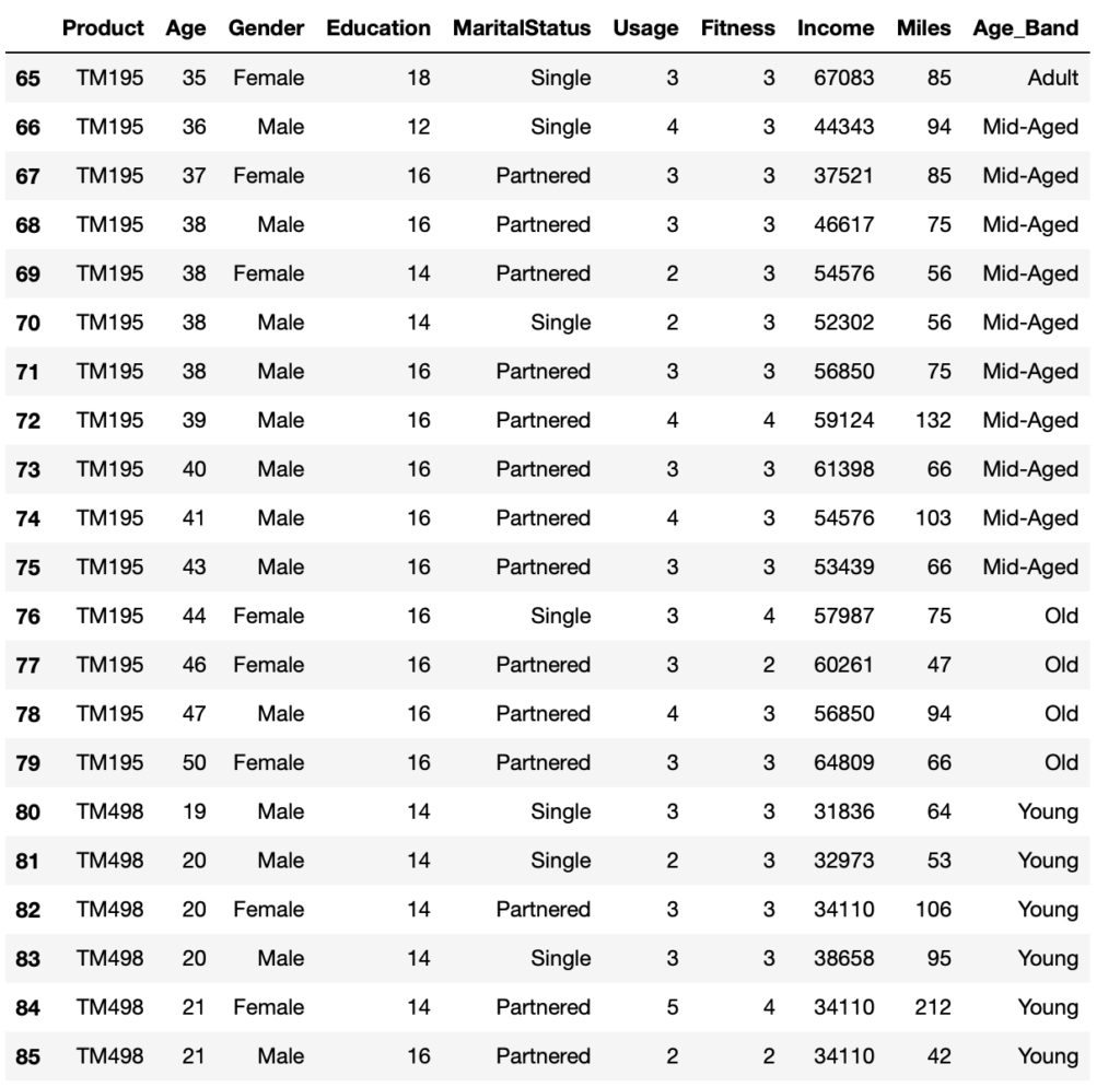
You can easily add another column called ‘Age_Band’ that contains the different age brackets.

data['Age_Band'] = pd.cut(data['Age'], bins=[17, 25, 35, 43, 51], labels=['Young', 'Adult', 'Mid-Aged', 'Old'])

Now the dataset looks like below

data.loc[65:85, :]

2. Add a new column to the dataframe, based on certain conditions.

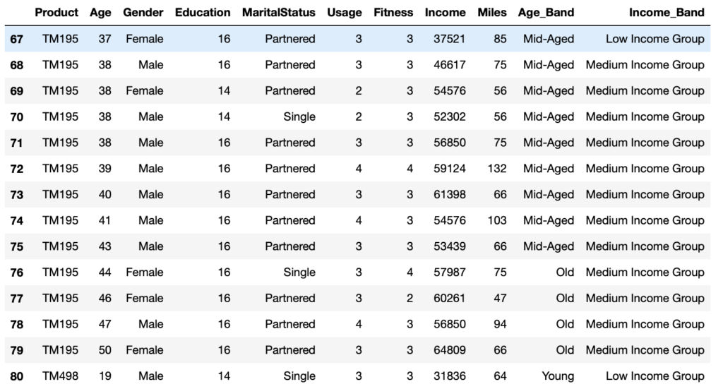
With reference to the same dataset as shown above, you can either use np.where or np.select to do the same.

data['Income_Band'] = np.where(
    data['Income'] < 40000 , "Low Income Group", np.where(
        (data['Income'] >=40000) & (data['Income'] < 80000), "Medium Income Group", np.where(
        data['Income'] >=80000, "High Income Group", np.nan)))

The same function can be achieved using np.select as below.

conditions = [
    data['Income'] < 40000,
    (data['Income'] >=40000) & (data['Income'] < 80000),
    data['Income'] >=80000
]
values = [
    "Low Income Group",
    "Medium Income Group",
    "High Income Group"
]
data['Income_Band'] = np.select(conditions, values)

This will lead to the below result.

data.loc[67:80, :]

3. Add a new column to the dataset, and copy it to another dataset, without affecting the original data.

data1 = data.assign(Age_New=data["Age"]*2)

Now, look how the original dataset remains unaffected, and a copy is created at the same time with the new column.

data.head()

data1.head()

4. Refer to the column names without using the dataframe

data.query('Age > 45')

data.query('Age > 30 & Age < 32')

2.2 Example of a practical analysis

Now, let’s analyse 3 datasets from a Movie Company, and create some useful insights.

1. rating.csv: It contains information on ratings given by the users to a particular movie.

2. movie.csv: The file contains information related to the movies and their genre.

3. user.csv: It contains information about the users who have rated the movies.

Let’s load all the datasets first.

movie = pd.read_csv("movie.csv")
ratings = pd.read_csv("ratings.csv")
user = pd.read_csv("user.csv")

Ensure that all the columns get displayed.

# Set the display option for max_columns to a high value
pd.options.display.max_columns = 999

Let’s look at how each data look like before going to the analysis.

movie.head(2)
ratings.head(2)
user.head(2)

Q1. How many rows are there for each datasets?

print(movie.shape)
print(ratings.shape)
print(user.shape)

(1680, 21)
(100000, 4)
(943, 5)

There are 1680 movies, 943 users and 100000 ratings.

Q2. What is the trend of the number of movies released after 1990?

To find this, let’s convert the “release date” column datatype into datetime format using the python’s datetime library. Then extract the year and store it in a new column called “year”

movie["year"] = pd.to_datetime(movie["release date"], dayfirst=True).dt.year
print(movie.head())

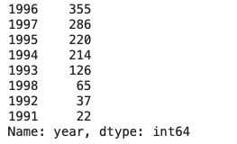
Now, we can find the number of movies released per year after 1990.

movie[movie['year'] > 1990]['year'].value_counts(ascending=False)

Insights

1. There was an upward trend of movies released after 1990
2. Most number of movies were released in the year 1996
3. Overall, from 1993 to 1996, majority of the movies were released

Q3. How many movies belong to a particular genre?

Here, we need to find the number of movies released under each genre e.g. Action or Adventure or Animation etc. Let’s extract all the columns with generes and sum up the numbers.

movie[movie.columns[3:-1]].sum().sort_values(ascending=False)

Insights

1. The most number of movies belong to the genre “Drama”
2. “Comedy”, “Action”, “Thriller” and “Romance” movies were second in number
3. “Adventure”, “Children’s”, “Crime” and “Sci-Fi” came next
4. Least number of movies were of type “Fantasy”, “Film-Noir”, “Western”, “Animation”, “Documentary” , “War”, “Musical”, “Mystery” and “Horror”

Q4. Which movies have more than one genre? 

We need to add up the total number of generes for each movie along the x-axis (axis=1) and store it in a new column “generes total”.

movie["generes total"] = movie[movie.columns[3:-1]].sum(axis=1)
movie[movie["generes total"] > 1][['movie title', 'generes total']].sort_values(ascending=False, by='generes total')

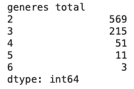
Let’s also aggregate the count of movies according to the “generes total”

movie[movie["generes total"] > 1][['generes total']].value_counts().sort_values(ascending=False)

Insights

1. There were 849 movies with more than one genere
2. 3 movies spanned across 6 generes
3. 569 movies, which is approximately 35% of the total, belongs to 2 generes

Q5. Which of the genres are most liked by the users?

There is no data for this in the movie dataset. So, we need to combine the ratings dataset along with the movie dataset.

# Merge the movie and the ratings datasets
merged = pd.merge(movie, ratings, on='movie id', how='inner')
# Extract the column names consisting of generes
generes = merged.columns[3:-3]
# Create a new DataFrame with the genere columns
df = pd.DataFrame(columns=generes)
# Populate the data frame with the ratings, wherever the genere is 1
for i in generes:
  df[i] = np.where(merged[i] == 1, merged['rating'], np.nan)
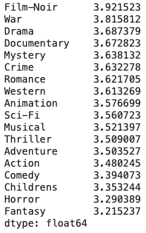
# Display the mean of the ratings for each of the generes
df.mean().sort_values(ascending=False)

Insights

1. “Film-Noir” genere has the highest ratings, however, there are only 24 movies in that category
2. Hence, the company needs to increase its collection of movies in the genere “Film-Noir”
3. Same logic applies to the movies with “War” genere. The company needs to increate the number of “War” movies.
4. Same applies to “Crime”, “Documentary” and “Mystery” movies

Q6. Which of the movies have been most rated by the users?

merged.groupby('movie title')['rating'].mean().sort_values(ascending=False).head(20)

Hear, we see all the movies that are rated 5.0

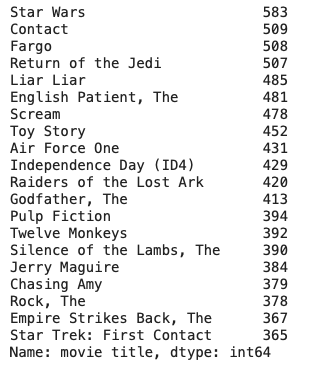
Q7. What are the top 10 movies that have received most rating counts?

merged['movie title'].value_counts().head(20)

Q8. Compare the movies with highest count of rating with the mean ratings.

First, get a Series with the ratings against movie titles and create a new data frame with that data.

s_rating = merged.groupby('movie title')['rating'].mean().sort_values(ascending=False)
dff1 = pd.DataFrame(s_rating, columns=['rating'])

Then, get a Series with the count of ratings against the movie titles and create a new data frame with that data.

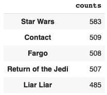
s_ratingcounts = merged['movie title'].value_counts()
dff2 = pd.DataFrame(s_ratingcounts)
dff2.rename(columns={'movie title': "counts"}, inplace=True)

dff1.head()

dff2.head()

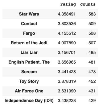
Now, merge the two data frames based on the indexes.

pd.merge(dff1, dff2, left_index=True, right_index=True).sort_values(by='counts', ascending=False).head(10)

Q9. Is there any relationship between demographic details of the users and ratings for the movies? 

We need to merge the rating and the user datasets.

user_rating_data = pd.merge(user, ratings, how="inner", on='user id')

user_rating_data.head()

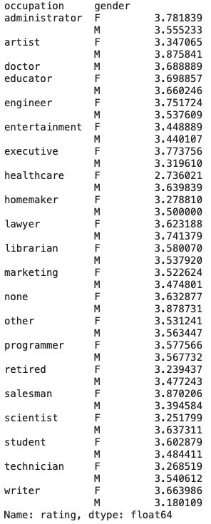
Now, calculate the mean ratings based on occupation and also between male and female in each occupation.

user_rating_data.groupby(['occupation', 'gender'])['rating'].mean()

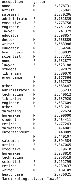
Let’s now sort based on the mean ratings.

user_rating_data.groupby(['occupation', 'gender'])['rating'].mean().sort_values(ascending=False)

Insights

1. The highest ratings are given by the ones without any occupation i.e those males without any jobs.
2. The lowest ratings are given by Female healthcare workers

Below are the files/datasets you can use to perform the above analysis